
Understanding Micro, Macro, and Weighted Averages for Scikit-Learn metrics in multi-class classification with example
2022-06-19Steps to package and publish Python codes to PyPI (pip)
2022-07-28Maximum Likelihood Estimation (MLE) and Maximum A Posteriori (MAP), are both methods for estimating variable from probability distributions or graphical models. They are similar, as they compute a single estimate, instead of a full distribution.
MLE, as a data scientist who has already indulged ourselves in Machine Learning, would be familiar with the method. It is so often used that sometimes people might even use it without knowing it. For example, when fitting a Gaussian distribution, we immediately take the sample mean and sample variance and use it as the parameter of our Gaussian. This is MLE, as, if we take the derivative of the Gaussian function with respect to the mean and variance, and maximise it by making the derivative to zero, what we get is functions that are calculating the sample mean and sample variance.
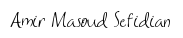
Speaking in more abstract terms, let’s say we have a likelihood function P(X|θ). Then, the MLE for θ, the parameter we want to infer, is:
As taking a product of some numbers less than 1 would approach 0 as the number of those numbers goes to infinity, it would be not practical to compute. Hence, we will instead work in the log space, as the logarithm is monotonically increasing, so maximizing a function is equal to maximizing the log of that function.

In order to use this framework, we just need to derive the log-likelihood of our model, then maximizing it with regard to θ using our favorite optimization algorithm (e.g. Gradient Descent).
Up to this point, we now understand what does MLE does. From here, we could draw a parallel line with MAP estimation.
MAP usually comes up in Bayesian setting. As the name suggests, it works on a posterior distribution, not only the likelihood.
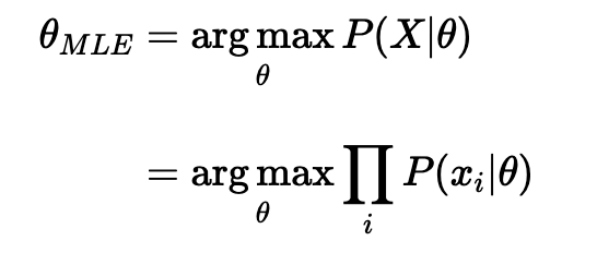
Recall the Bayes’ rule, we could get the posterior as a product of likelihood and prior:

We ignore the normalizing constant as we are strictly speaking about optimization here, so proportionality should be sufficient.
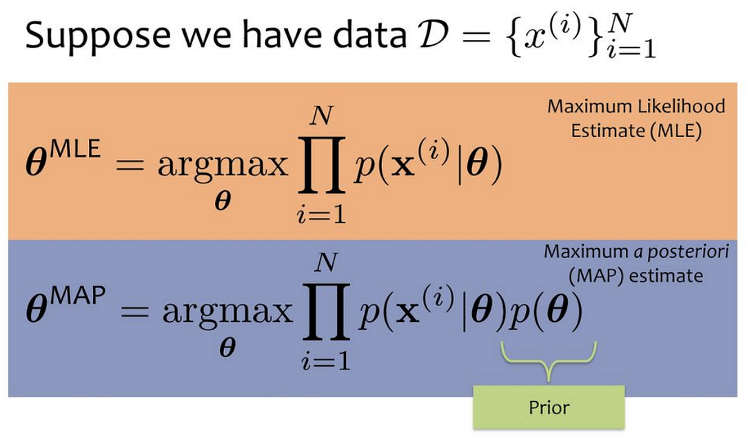
If we replace the likelihood in the MLE formula above with the posterior, we can get:
Comparing both MLE and MAP equations, the only thing that differs is the inclusion of prior P(θ) in MAP, otherwise, they are identical. What it means is that the likelihood is now weighted with some weight coming from the prior.
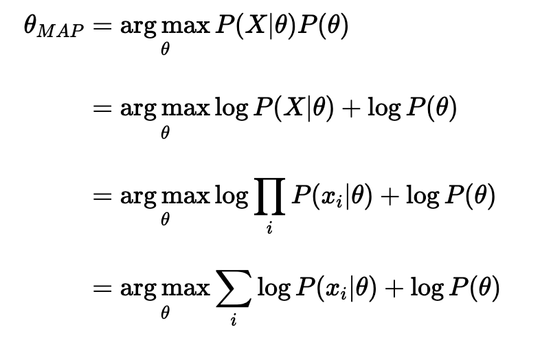
Let’s consider what if we use the simplest prior in our MAP estimation, say uniform prior. This means we can assign equal weights everywhere, on all possible values of the θ. The implication is that the likelihood is equivalently weighted by some constants. Being constant, it could be ignored from our MAP equation, as it will not contribute to the max.
Let’s be more concrete, let’s say we could assign six possible values into θ. Now, our prior P(θ) is 1/6 everywhere in the distribution. And consequently, we could ignore that constant in our MAP estimation.
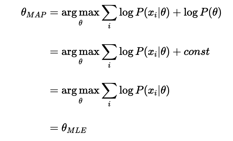
As it shows, we are back at the MLE equation!
If we choose a different prior other than uniform, say a Gaussian one instead, then the prior is no longer a constant anymore. The probability is likely to be high or low but won’t be the same, as this depends on the region of the distribution.
So clearly we can draw the conclusion: MLE is a special case of MAP when the prior is uniform.
References: