Steps to setup PyTorch with GPU for NVIDIA GTX 960m (Asus VivoBook n552vw) in Ubuntu
2020-11-20
Handling cyclical features, such as hours in a day, for machine learning pipelines with Python example
2021-03-26Policy gradients
Policy gradients is a family of algorithms for solving reinforcement learning problems by directly optimizing the policy in the policy space. This is in stark contrast to value-based approaches (such as Q-learning used in Learning Atari games by DeepMind. Policy gradients have several appealing properties, for one they produce stochastic policies (by learning a probability distribution over actions given observations) whereas value-based approaches are deterministic as they will typically choose actions greedily with respect to the value function being learned which can lead to under-exploration (one needs to introduce exploration strategies such as ϵ-greedy explicitly to get around this). Another advantage of policy gradients is their ability to tackle continuous action spaces without discretization which is necessary for value-based methods. This is not to say that value-based approaches are useless, one of the biggest disadvantages of policy gradients is their high variance estimates of the gradient updates. This leads to very noisy gradient estimates and can destabilize the learning process. I think it is fair to say that a lot of reinforcement learning research with policy gradients in the past few years has been about trying to reduce the variance of these gradient updates to improve the trainability of these algorithms. It is also worth mentioning that in state-of-the-art implementations and tasks, it is common to use the so-called actor-critic algorithms which include a policy gradient and a value function estimator to combine the best properties of both approaches.
Policy-Gradient methods are a subclass of Policy-Based methods that estimate an optimal policy’s weights through gradient ascent.

Intuitively, gradient ascent begins with an initial guess for the value of the policy’s weights that maximizes the expected return, then, the algorithm evaluates the gradient at that point that indicates the direction of the steepest increase of the function of expected return, and so we can make a small step in that direction. We hope that we end up at a new value of the policy’s weights for which the value of the expected return function is a little bit larger. The algorithm then repeats this process of evaluating the gradient and taking steps until it considers that it is eventually reached the maximum expected return.
You can find the codes for this post on my Github.
Introduction
Policy-based methods can learn either stochastic or deterministic policies. With a stochastic policy, our neural network’s output is an action vector that represents a probability distribution (rather than returning a single deterministic action).
The policy we will follow in the new method presented in this Post is selecting an action from this probability distribution. This means that if our Agent ends up in the same state twice, we may not end up taking the same action every time. Such representation of actions as probabilities has many advantages, for instance, the advantage of smooth representation: if we change our network weights a bit, the output of the neural network will change, but probably just a little bit.
In the case of a deterministic policy, with a discrete output, even a small adjustment of the weights can lead to a jump to a different action. However, if the output is a probability distribution, a small change of weights will usually lead to a small change in output distribution. This is a very important property due gradient optimization methods are all about tweaking the parameters of a model a bit to improve the results.
But how can be changed network’s parameters to improve the policy?
The key idea underlying policy gradients is reinforcing good actions: to push up the probabilities of actions that lead to higher returns, and push down the probabilities of actions that lead to a lower return, until you arrive at the optimal policy. The policy gradient method will iteratively amend the policy network weights (with smooth updates) to make state-action pairs that resulted in positive return more likely, and make state-action pairs that resulted in negative return less likely.
To introduce this idea I will start with a vanilla version (the basic version) of the policy gradient method called REINFORCE algorithm (original paper). This algorithm is the fundamental policy gradient algorithm on which nearly all the advanced policy gradient algorithms are based.
REINFORCE: Mathematical definitions
Let’s look at a more mathematical definition of the algorithm since it will be good for us in order to understand the most advanced algorithms in the following Posts.
Trajectory
The first thing we need to define is a trajectory, just a state-action-rewards sequence (but we ignore the reward). A trajectory is a little bit more flexible than an episode because there are no restrictions on its length; it can correspond to a full episode or just a part of an episode. We denote the length with a capital H, where H stands for Horizon, and we represent a trajectory with τ:

The method REINFORCE is built upon trajectories instead of episodes because maximizing expected return over trajectories (instead of episodes) lets the method search for optimal policies for both episodic and continuing tasks.
Although for the vast majority of episodic tasks, where a reward is only delivered at the end of the episode, it only makes sense just to use the full episode as a trajectory; otherwise, we don’t have enough reward information to meaningfully estimate the expected return.
Return of a trajectory
We denote the return for a trajectory τ with R(τ), and it is calculated as the sum reward from that trajectory τ:

The parameter Gk is called the total return, or future return, at time step k for the transition k

It is the return we expect to collect from time step k until the end of the trajectory, and it can be approximated by adding the rewards from some state in the episode until the end of the episode using gamma γ:

Remember that the goal of this algorithm is to find the weights θ of the neural network that maximizes the expected return that we denote by U(θ) and can be defined as:

To see how it corresponds to the expected return, note that we have expressed the return R(τ) as a function of the trajectory τ. Then, we calculate the weighted average, where the weights are given by P(τ;θ), the probability of each possible trajectory, of all possible values that the return R(τ) can take. Note that probability depends on the weights θ in the neural network because θ defines the policy used to select the actions in the trajectory, which also plays a role in determining the states that the agent observes.
Gradient ascent
As I already introduced, one way to determine the value of θ that maximizes U(θ) function is through gradient ascent.
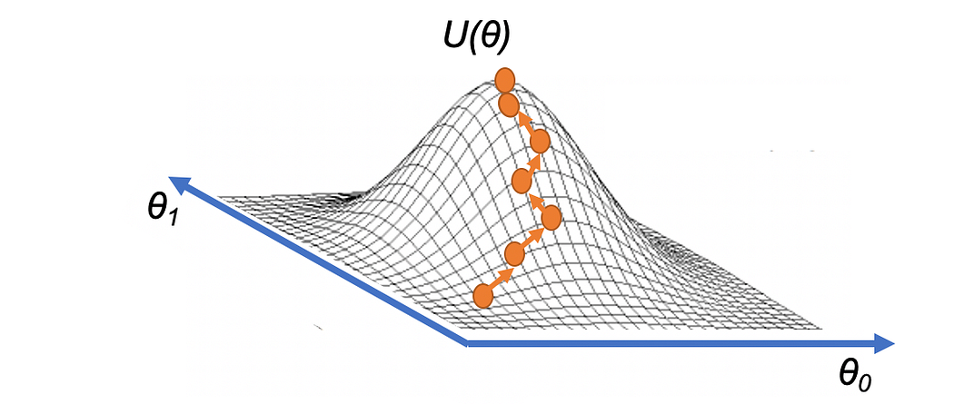
Equivalent to the Hill-Climbing algorithm presented in this Post, intuitively we can visualize that the gradient ascent draws up a strategy to reach the highest point of a hill, U(θ), just iteratively taking small steps in the direction of the gradient:

source: https://torres.ai
Mathematically, our update step for gradient ascent can be expressed as:

where α is the step size that is generally allowed to decay over time (equivalent to the learning rate decay in deep learning). Once we know how to calculate or estimate this gradient, we can repeatedly apply this update step, in the hopes that θ converges to the value that maximizes U(θ).
Gradient ascent is closely related to gradient descent, where the differences are that gradient descent is designed to find the minimum of a function (steps in the direction of the negative gradient), whereas gradient ascent will find the maximum (steps in the direction of the gradient). I will use this approach in our code in PyTorch.
Sampling and estimate
To apply this method, we will need to be able to calculate the gradient ∇U(θ); however, we won’t be able to calculate the exact value of the gradient since that is computationally too expensive because, to calculate the gradient exactly, we’ll have to consider every possible trajectory, becoming an intractable problem in most cases.
Instead of doing this, the method samples trajectories using the policy and then uses those trajectories only to estimate the gradient. This sampling is equivalent to the approach of Monte Carlo presented in this post, and for this reason, the method REINFORCE is also known as Monte Carlo Policy Gradients.
Pseudocode
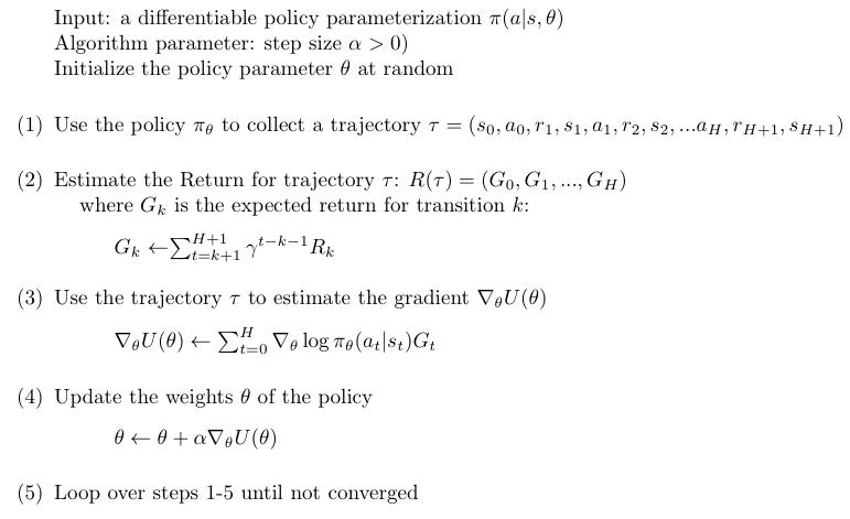
In summary, the pseudocode that describes in more detail the behavior of this method can be written as:

Let’s look a bit more closely at the equation of step 3 in the pseudocode to understand it. I begin by making some simplifying assumptions, for example, assuming that corresponds to a full episode.
Remember that R(τ) is just the cumulative rewards from the trajectory τ (the only one trajectory) at each time step. Assume that the reward signal at time step t and the sample play we are working with gives the Agent a reward of positive one (Gt=+1) if we won the game and a reward of negative one (Gt=-1) if we lost. On the other hand, the term

looks at the probability that the Agent selects action at from state st in time step t. Remember that π with the subscript θ refers to the policy which is parameterized by θ. Then, the full expression takes the gradient of the log of that probability is

This will tell us how we should change the weights of the policy θ if we want to increase the log probability of selecting action at from state st. Specifically, suppose we nudge the policy weights by taking a small step in the direction of this gradient. In that case, it will increase the log probability of selecting the action from that state, and if we step in the opposite direction will decrease the log probability.
The following equation will do all of these updates all at once for each state-action pair, at and st, at each time step t in the trajectory:

To see this behavior, assume that the Agent won the episode. Then, Gt is just a positive one (+1), and what the sum does is add up all the gradient directions we should step in to increase the log probability of selecting each state-action pair. That’s equivalent to just taking H+1 simultaneous steps where each step corresponds to a state-action pair in the trajectory.
On the opposite, if the Agent lost, Gt becomes a negative one, which ensures that instead of stepping in the direction of the steepest increase of the log probabilities, the method steps in the direction of the steepest decrease.
The proof of how to derive the equation that approximates the gradient can be safely skipped, what interests us much more is the meaning of the expression.
Why optimize log probability instead of probability
In Gradient methods where we can formulate some probability p that should be maximized, we would actually optimize the log probability log(p) instead of the probability p for some parameters theta.
The reason is that generally, works better to optimize log(p) than p due to the gradient of log(p) is generally more well-scaled. Remember that probabilities are bounded by 0 and 1 by definition, so the range of values that the optimizer can operate over is limited and small.
In this case, sometimes probabilities may be extremely tiny or very close to 1, and this runs into numerical issues when optimizing on a computer with limited numerical precision. If we instead use a surrogate objective, namely log(p) (natural logarithm), we have an objective that has a larger “dynamic range” than raw probability space, since the log of probability space ranges from (-∞,0), and this makes the log probability easier to compute.
Coding REINFORCE
Now, we will explore an implementation of the REINFORCE to solve OpenAI Gym’s Cartpole environment.
The entire code of this post can be found on GitHub and can be run as a Colab google notebook using this link.
Initializations
First, I will import all necessary packages with the following lines of code:
import numpy as np
import torch
import gym
from matplotlib import pyplot as plt
And also the OpenAI Gym’s Cartpole Environment:
env = gym.make('CartPole-v0')
Policy Network
I will build a neural network that serves as a policy network. The policy network will accept a state vector as input, and it will produce a (discrete) probability distribution over the possible actions.
obs_size = env.observation_space.shape[0]
n_actions = env.action_space.n
HIDDEN_SIZE = 256

model = torch.nn.Sequential(
             torch.nn.Linear(obs_size, HIDDEN_SIZE),
             torch.nn.ReLU(),
             torch.nn.Linear(HIDDEN_SIZE, n_actions),
             torch.nn.Softmax(dim=0)
     )
The model is only two linear layers, with a ReLU activation function for the first layer, and the Softmax function for the last layer. By default, the initialization is with random weights).
print (model)

With the result of the neural network, the Agent samples from the probability distribution to take an action that will be executed in the Environment.
 act_prob = model(torch.from_numpy(curr_state).float())
action = np.random.choice(np.array([0,1]), p=act_prob.data.numpy())
prev_state = curr_state
curr_state, _, done, info = env.step(action)
The second line of this code samples an action from the probability distribution produced by the policy network obtained in the first line. Then in the last line of this code, the Agent takes the action.
The training loop
The training loop trains the policy network by updating the parameters θ. The following pseudocode describes in the previous section.
First, I define the optimizer and initialize some variables:
learning_rate = 0.003
optimizer = torch.optim.Adam(model.parameters(), lr=learning_rate)

Horizon = 500
MAX_TRAJECTORIES = 500
gamma = 0.99
score = []
where is learning_rate is the step size α, Horizon is the H and gammais γ in the previous pseudocode. Using these variables, the main loop with the number of iterations is defined by MAX_TRAJECTORIESis coded as:
for trajectory in range(MAX_TRAJECTORIES):
    curr_state = env.reset()
    done = False
    transitions = []

    for t in range(Horizon):
        act_prob = model(torch.from_numpy(curr_state).float())
        action = np.random.choice(np.array([0,1]), p=act_prob.data.numpy())
        prev_state = curr_state
        curr_state, _, done, info = env.step(action)
        transitions.append((prev_state, action, t+1))
        if done:
            break
    score.append(len(transitions))
    reward_batch = torch.Tensor([r for (s,a,r) in transitions]).flip(dims=(0,))

    batch_Gvals =[]
    for i in range(len(transitions)):
        new_Gval=0
        power=0
        for j in range(i,len(transitions)):
             new_Gval=new_Gval+((gamma**power)*reward_batch[j]).numpy()
             power+=1
        batch_Gvals.append(new_Gval)
    expected_returns_batch=torch.FloatTensor(batch_Gvals)


    expected_returns_batch /= expected_returns_batch.max()

    state_batch = torch.Tensor([s for (s,a,r) in transitions])
    action_batch = torch.Tensor([a for (s,a,r) in transitions])

    pred_batch = model(state_batch)
    prob_batch = pred_batch.gather(dim=1,index=action_batch.long().view(-1,1)).squeeze()

    loss = - torch.sum(torch.log(prob_batch) * expected_returns_batch)

    optimizer.zero_grad()
    loss.backward()
    optimizer.step()
With score list we will keep track of the trajectory length over training time. We keep track of the actions and states in the list transactions for the transactions of the current trajectory.
Following we compute the expected return for each transaction (code snippet from the previous listing):
    for i in range(len(transitions)):
        new_Gval=0
        power=0
        for j in range(i,len(transitions)):
             new_Gval=new_Gval+((gamma**power)*reward_batch[j]).numpy()
             power+=1
        batch_Gvals.append(new_Gval)
    expected_returns_batch=torch.FloatTensor(batch_Gvals)
    expected_returns_batch /= expected_returns_batch.max()
The listbatch_Gvals is used to compute the expected return for each transaction as it is indicated in the previous pseudocode. The list expected_return stores the expected returns for all the transactions of the current trajectory. Finally, this code normalizes the rewards to be within the [0,1] interval to improve numerical stability.
The loss function requires an array of action probabilities, prob_batch, for the actions that were taken and the discounted rewards:
loss = - torch.sum(torch.log(prob_batch) * expected_returns_batch)
For this purpose we recompute the action probabilities for all the states in the trajectory and subsets the action probabilities associated with the actions that were actually taken with the following two lines of code:
pred_batch = model(state_batch)
prob_batch = pred_batch.gather(dim=1,index=action_batch.long().view(-1,1)).squeeze()
An important detail is the minus sign in the loss function of this code:
loss= -torch.sum(torch.log(prob_batch)*expected_returns_batch)
Why do we introduce a – in the log_prob? In general, we prefer to set things up so that we are minimizing an objective function instead of maximizing since it plays nicely with PyTorch’s built-in optimizers (using stochastic gradient descent). We should instead tell PyTorch to minimize 1-π. This loss function approaches 0 as π nears 1, so we are encouraging the gradients to maximize π for the action we took.
Also, let’s remember that we use a surrogate objective, namely –log π (where the log is the natural logarithm), because we have an objective that has a larger dynamic range than raw probability space (bounded by 0 and 1 by definition), since the log of probability space ranges from (–∞,0), and this makes the log probability easier to compute.
Finally, mention that we included in the code the following lines of code to control the progress of the training loop:
    if trajectory % 50 == 0 and trajectory>0:
            print('Trajectory {}\tAverage Score: {:.2f}'.format(trajectory, np.mean(score[-50:-1])))

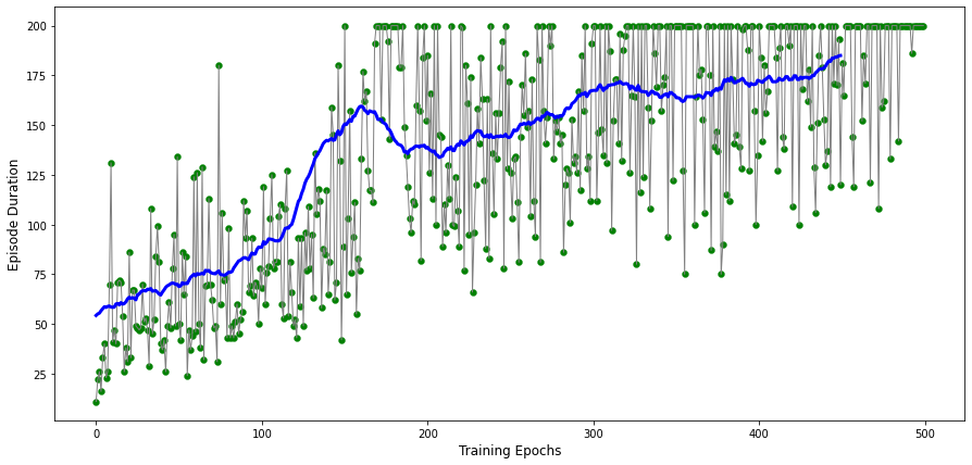
We can visualize the results of this code by running the following code:
def running_mean(x):
    N=50
    kernel = np.ones(N)
    conv_len = x.shape[0]-N
    y = np.zeros(conv_len)
    for i in range(conv_len):
        y[i] = kernel @ x[i:i+N]
        y[i] /= N
    return y


score = np.array(score)
avg_score = running_mean(score)

plt.figure(figsize=(15,7))
plt.ylabel("Trajectory Duration",fontsize=12)
plt.xlabel("Training Epochs",fontsize=12)
plt.plot(score, color='gray' , linewidth=1)
plt.plot(avg_score, color='blue', linewidth=3)
plt.scatter(np.arange(score.shape[0]),score, color='green' , linewidth=0.3)
You should be able to obtain a plot with a nicely increasing trend of the trajectory duration.

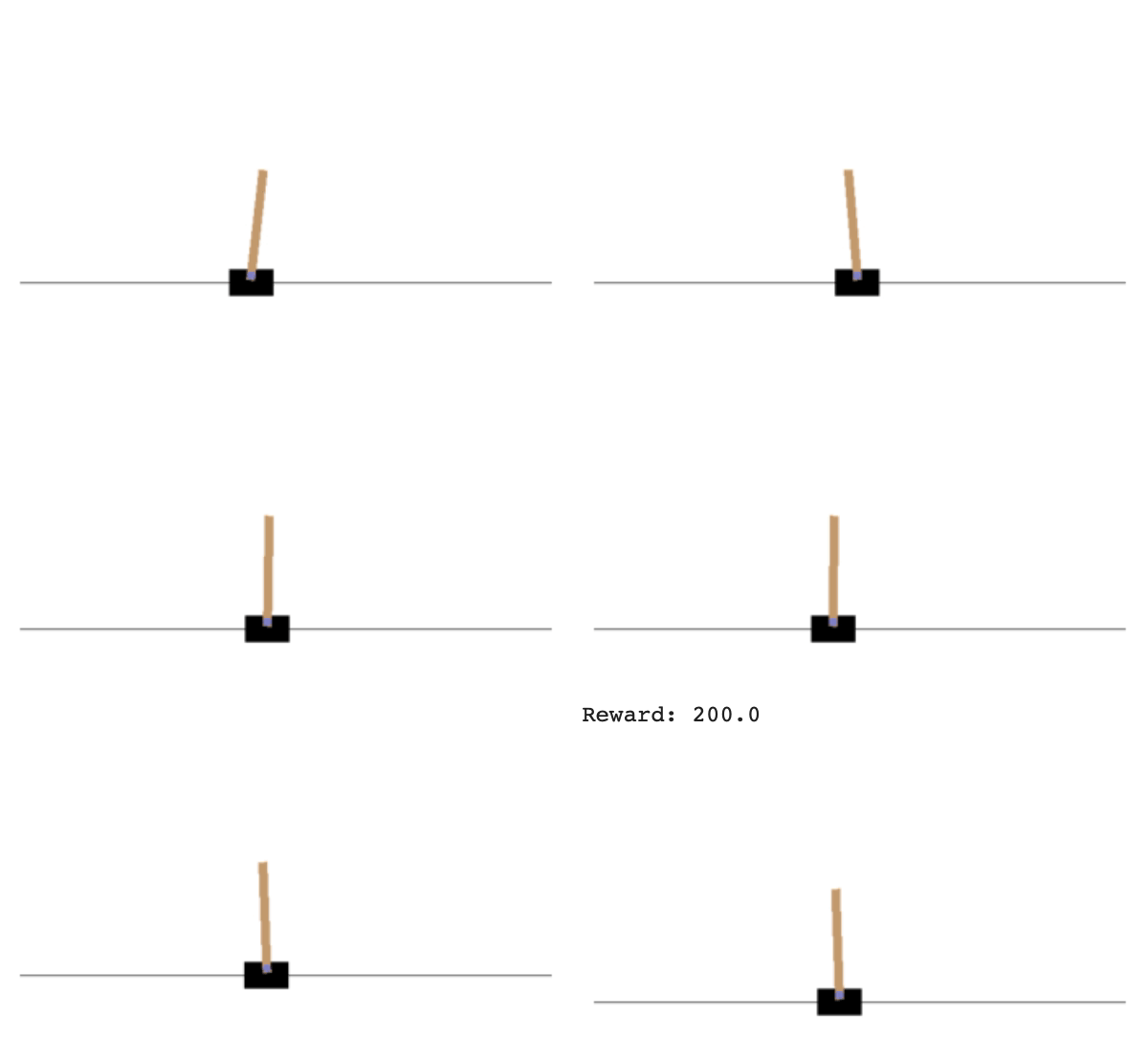
We also can render how the Agent applies the policy with the following code:
def watch_agent():
  env = gym.make('CartPole-v0')
  state = env.reset()
  rewards = []
  img = plt.imshow(env.render(mode='rgb_array'))
  for t in range(2000):
    pred = model(torch.from_numpy(state).float())
    action = np.random.choice(np.array([0,1]), p=pred.data.numpy())

    img.set_data(env.render(mode='rgb_array'))
    plt.axis('off')
    display.display(plt.gcf())
    display.clear_output(wait=True)

    state, reward, done, _ = env.step(action)
    rewards.append(reward)
    if done:
        print("Reward:", sum([r for r in rewards]))
        break
  env.close()

watch_agent()

Policy-based versus Value-based methods
Now that we know the two families of methods, what are the main differences between them?
- Policy methods, such as REINFORCE, directly optimize the policy. Value methods, such as DQN, do the same indirectly, learning the value first and, obtaining the policy based on this value.
- Policy methods are on-policy and require fresh samples from the Environment (obtained with the policy). Instead, Value methods can benefit from old data obtained from the old policy.
- Policy methods are usually less sample-efficient, which means they require more interaction with the Environment. Remember that value methods can benefit from large replay buffers.
Policy methods will be the more natural choice in some situations, and in other situations, value methods will be a better option.
Summary
In this post, we have explained in detail the REINFORCE algorithm, and we have coded it. As a stochastic gradient method, REINFORCE works well in simple problems and has good theoretical convergence properties.
References:
https://www.janisklaise.com/post/rl-policy-gradients/
https://towardsdatascience.com/policy-gradient-reinforce-algorithm-with-baseline-e95ace11c1c4
https://medium.com/@thechrisyoon/deriving-policy-gradients-and-implementing-reinforce-f887949bd63
https://julien-vitay.net/deeprl/PolicyGradient.html
https://towardsdatascience.com/policy-gradient-methods-104c783251e0

2 Comments
Hi, what should we put as curr_state on “act_prob = model(torch.from_numpy(curr_state).float())”?
Hi Ryan,
You don’t need to run this segment of code alone. Please see that this piece of code is used within the following “The training loop” section and I provided it to explain the steps. You can also get the code from: https://gist.github.com/iamirmasoud/5712ea4bf5256f2c6adb59d137dae6e1