
Setup collaborative MLflow with PostgreSQL as Tracking Server and MinIO as Artifact Store using docker containers
2022-08-30Guidelines to use Transfer Learning in Convolutional Neural Networks
2022-09-20Understand Q-Learning in Reinforcement Learning with a numerical example and Python implementation
This tutorial introduces the concept of Q-learning through a simple but comprehensive numerical example. The example describes an agent which uses unsupervised training to learn about an unknown environment. You might also find it helpful to compare this example with the accompanying source code examples.
Suppose we have 5 rooms in a building connected by doors as shown in the figure below. We’ll number each room from 0 through 4. The outside of the building can be thought of as one big room (5). Notice that doors 1 and 4 lead into the building from room 5 (outside).

We can represent the rooms on a graph, each room as a node, and each door as a link.

For this example, we’d like to put an agent in any room, and from that room, go outside the building (this will be our target room). In other words, the goal room is number 5. To set this room as a goal, we’ll associate a reward value to each door (i.e. link between nodes). The doors that lead immediately to the goal have an instant reward of 100. Other doors not directly connected to the target room have zero rewards. Because doors are two-way ( 0 leads to 4, and 4 leads back to 0 ), two arrows are assigned to each room. Each arrow contains an instant reward value, as shown below:

Of course, Room 5 loops back to itself with a reward of 100, and all other direct connections to the goal room carry a reward of 100. In Q-learning, the goal is to reach the state with the highest reward, so that if the agent arrives at the goal, it will remain there forever. This type of goal is called an “absorbing goal”.
Imagine our agent as a dumb virtual robot that can learn through experience. The agent can pass from one room to another but has no knowledge of the environment, and doesn’t know which sequence of doors leads to the outside.
Suppose we want to model some kind of simple evacuation of an agent from any room in the building. Now suppose we have an agent in Room 2 and we want the agent to learn to reach outside the house (5).

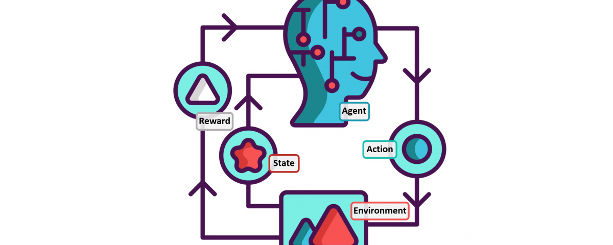
The terminology in Q-Learning includes the terms “state” and “action”.
We’ll call each room, including outside, a “state”, and the agent’s movement from one room to another will be an “action”. In our diagram, a “state” is depicted as a node, while “action” is represented by the arrows.

Suppose the agent is in state 2. From state 2, it can go to state 3 because state 2 is connected to 3. From state 2, however, the agent cannot directly go to state 1 because there is no direct door connecting rooms 1 and 2 (thus, no arrows). From state 3, it can go either to state 1 or 4 or back to 2 (look at all the arrows about state 3). If the agent is in state 4, then the three possible actions are to go to states 0, 5, or 3. If the agent is in state 1, it can go either to state 5 or 3. From state 0, it can only go back to state 4.
We can put the state diagram and the instant reward values into the following reward table, “matrix R”.

The -1’s in the table represent null values (i.e.; where there isn’t a link between nodes). For example, State 0 cannot go to State 1.
Now we’ll add a similar matrix, “Q”, to the brain of our agent, representing the memory of what the agent has learned through experience. The rows of matrix Q represent the current state of the agent, and the columns represent the possible actions leading to the next state (the links between the nodes).
The agent starts out knowing nothing, the matrix Q is initialized to zero. In this example, for the simplicity of explanation, we assume the number of states is known (to be six). If we didn’t know how many states were involved, the matrix Q could start with only one element. It is a simple task to add more columns and rows in matrix Q if a new state is found.
The transition rule of Q learning is a very simple formula:
Q(state, action) = R(state, action) + Gamma * Max[Q(next state, all actions)]
According to this formula, a value assigned to a specific element of matrix Q is equal to the sum of the corresponding value in matrix R and the learning parameter Gamma, multiplied by the maximum value of Q for all possible actions in the next state.
Our virtual agent will learn through experience, without a teacher (this is called unsupervised learning). The agent will explore from state to state until it reaches the goal. We’ll call each exploration an episode. Each episode consists of the agent moving from the initial state to the goal state. Each time the agent arrives at the goal state, the program goes to the next episode.
The Q-Learning algorithm goes as follows:
1. Set the gamma parameter and environment rewards in matrix R.
2. Initialize matrix Q to zero.
3. For each episode:
Select a random initial state.
Do While the goal state hasn’t been reached.
- Select one among all possible actions for the current state.
- Using this possible action, consider going to the next state.
- Get maximum Q value for this next state based on all possible actions.
- Compute: Q(state, action) = R(state, action) + Gamma * Max[Q(next state, all actions)]
- Set the next state as the current state.
End Do
End For
The algorithm above is used by the agent to learn from experience. Each episode is equivalent to one training session. In each training session, the agent explores the environment (represented by matrix R ) and receives the reward (if any) until it reaches the goal state. The purpose of the training is to enhance the ‘brain’ of our agent, represented by matrix Q. More training results in a more optimized matrix Q. In this case, if the matrix Q has been enhanced, instead of exploring around, and going back and forth to the same rooms, the agent will find the fastest route to the goal state.
The Gamma parameter has a range of 0 to 1 (0 <= Gamma > 1). If Gamma is closer to zero, the agent will tend to consider only immediate rewards. If Gamma is closer to one, the agent will consider future rewards with greater weight, willing to delay the reward.
To use the matrix Q, the agent simply traces the sequence of states, from the initial state to the goal state. The algorithm finds the actions with the highest reward values recorded in matrix Q for the current state:
Algorithm to utilize the Q matrix:
- Set current state = initial state.
- From the current state, find the action with the highest Q value.
- Set current state = next state.
- Repeat Steps 2 and 3 until current state = goal state.
The algorithm above will return the sequence of states from the initial state to the goal state.
Q-Learning Example By Hand
To understand how the Q-learning algorithm works, we’ll go through a few episodes step by step. The rest of the steps are illustrated in the source code examples.
We’ll start by setting the value of the learning parameter Gamma = 0.8, and the initial state as Room 1.
Initialize matrix Q as a zero matrix:

Look at the second row (state 1) of matrix R. There are two possible actions for the current state 1: go to state 3, or go to state 5. By random selection, we select to go to 5 as our action.
Now let’s imagine what would happen if our agent were in state 5. Look at the sixth row of the reward matrix R (i.e. state 5). It has 3 possible actions: go to states 1, 4, or 5.
Q(state, action) = R(state, action) + Gamma * Max[Q(next state, all actions)]
Q(1, 5) = R(1, 5) + 0.8 * Max[Q(5, 1), Q(5, 4), Q(5, 5)] = 100 + 0.8 * 0 = 100
Since matrix Q is still initialized to zero, Q(5, 1), Q(5, 4), Q(5, 5), are all zero. The result of this computation for Q(1, 5) is 100 because of the instant reward from R(5, 1).
The next state, 5, now becomes the current state. Because 5 is the goal state, we’ve finished one episode. Our agent’s brain now contains an updated matrix Q as:

For the next episode, we start with a randomly chosen initial state. This time, we have state 3 as our initial state.
Look at the fourth row of matrix R; it has 3 possible actions: go to states 1, 2, or 4. By random selection, we select to go to state 1 as our action.
Now we imagine that we are in state 1. Look at the second row of reward matrix R (i.e. state 1). It has 2 possible actions: go to state 3 or state 5. Then, we compute the Q value:
Q(state, action) = R(state, action) + Gamma * Max[Q(next state, all actions)]
Q(1, 5) = R(1, 5) + 0.8 * Max[Q(1, 2), Q(1, 5)] = 0 + 0.8 * Max(0, 100) = 80
We use the updated matrix Q from the last episode. Q(1, 3) = 0 and Q(1, 5) = 100. The result of the computation is Q(3, 1) = 80 because the reward is zero. The matrix Q becomes:

The next state, 1, now becomes the current state. We repeat the inner loop of the Q learning algorithm because state 1 is not the goal state.
So, starting the new loop with the current state 1, there are two possible actions: go to state 3, or go to state 5. By lucky draw, our action selected is 5.
Now, imagine we’re in state 5, there are three possible actions: go to state 1, 4, or 5. We compute the Q value using the maximum value of these possible actions.
Q(state, action) = R(state, action) + Gamma * Max[Q(next state, all actions)]
Q(1, 5) = R(1, 5) + 0.8 * Max[Q(5, 1), Q(5, 4), Q(5, 5)] = 100 + 0.8 * 0 = 100
The updated entries of matrix Q, Q(5, 1), Q(5, 4), and Q(5, 5), are all zero. The result of this computation for Q(1, 5) is 100 because of the instant reward from R(5, 1). This result does not change the Q matrix.
Because 5 is the goal state, we finish this episode. Our agent’s brain now contains updated matrix Q as:
If our agent learns more through further episodes, it will finally reach convergence values in matrix Q like:

This matrix Q, can then be normalized (i.e.; converted to a percentage) by dividing all non-zero entries by the highest number (500 in this case):

Once the matrix Q gets close enough to a state of convergence, we know our agent has learned the most optimal paths to the goal state. Tracing the best sequences of states is as simple as following the links with the highest values at each state.

For example, from initial State 2, the agent can use the matrix Q as a guide:
From State 2 the maximum Q values suggest the action to go to state 3.
From State 3 the maximum Q values suggest two alternatives: go to state 1 or 4. Suppose we arbitrarily choose to go to 1.
From State 1 the maximum Q values suggest the action to go to state 5.
Thus the sequence is 2 – 3 – 1 – 5.
Python Implementation:
# Q-learning formula from http://sarvagyavaish.github.io/FlappyBirdRL/
# Visualization based on code from Gael Varoquaux gael.varoquaux@normalesup.org
# http://scikit-learn.org/stable/auto_examples/applications/plot_stock_market.html

import numpy as np
import matplotlib.pyplot as plt
from matplotlib.collections import LineCollection


# defines the reward/connection graph
r = np.array([[-1, -1, -1, -1,  0,  -1],
              [-1, -1, -1,  0, -1, 100],
              [-1, -1, -1,  0, -1,  -1],
              [-1,  0,  0, -1,  0,  -1],
              [ 0, -1, -1,  0, -1, 100],
              [-1,  0, -1, -1,  0, 100]]).astype("float32")
q = np.zeros_like(r)


def update_q(state, next_state, action, alpha, gamma):
    rsa = r[state, action]
    qsa = q[state, action]
    new_q = qsa + alpha * (rsa + gamma * max(q[next_state, :]) - qsa)
    q[state, action] = new_q
    # renormalize row to be between 0 and 1
    rn = q[state][q[state] > 0] / np.sum(q[state][q[state] > 0])
    q[state][q[state] > 0] = rn
    return r[state, action]


def show_traverse():
    # show all the greedy traversals
    for i in range(len(q)):
        current_state = i
        traverse = "%i -> " % current_state
        n_steps = 0
        while current_state != 5 and n_steps < 20:
            next_state = np.argmax(q[current_state])
            current_state = next_state
            traverse += "%i -> " % current_state
            n_steps = n_steps + 1
        # cut off final arrow
        traverse = traverse[:-4]
        print("Greedy traversal for starting state %i" % i)
        print(traverse)
        print("")


def show_q():
    # show all the valid/used transitions
    coords = np.array([[2, 2],
                       [4, 2],
                       [5, 3],
                       [4, 4],
                       [2, 4],
                       [5, 2]])
    # invert y axis for display
    coords[:, 1] = max(coords[:, 1]) - coords[:, 1]

    plt.figure(1, facecolor='w', figsize=(10, 8))
    plt.clf()
    ax = plt.axes([0., 0., 1., 1.])
    plt.axis('off')

    plt.scatter(coords[:, 0], coords[:, 1], c='r')

    start_idx, end_idx = np.where(q > 0)
    segments = [[coords[start], coords[stop]]
                for start, stop in zip(start_idx, end_idx)]
    values = np.array(q[q > 0])
    # bump up values for viz
    values = values
    lc = LineCollection(segments,
                        zorder=0, cmap=plt.cm.hot_r)
    lc.set_array(values)
    ax.add_collection(lc)

    verticalalignment = 'top'
    horizontalalignment = 'left'
    for i in range(len(coords)):
        x = coords[i][0]
        y = coords[i][1]
        name = str(i)
        if i == 1:
            y = y - .05
            x = x + .05
        elif i == 3:
            y = y - .05
            x = x + .05
        elif i == 4:
            y = y - .05
            x = x + .05
        else:
            y = y + .05
            x = x + .05

        plt.text(x, y, name, size=10,
                 horizontalalignment=horizontalalignment,
                 verticalalignment=verticalalignment,
                 bbox=dict(facecolor='w',
                           edgecolor=plt.cm.spectral(float(len(coords))),
                           alpha=.6))
    plt.show()

# Core algorithm
gamma = 0.8
alpha = 1.
n_episodes = 1E3
n_states = 6
n_actions = 6
epsilon = 0.05
random_state = np.random.RandomState(1999)
for e in range(int(n_episodes)):
    states = list(range(n_states))
    random_state.shuffle(states)
    current_state = states[0]
    goal = False
    if e % int(n_episodes / 10.) == 0 and e > 0:
        pass
        # uncomment this to see plots each monitoring
        #show_traverse()
        #show_q()
    while not goal:
        # epsilon greedy
        valid_moves = r[current_state] >= 0
        if random_state.rand() < epsilon:
            actions = np.array(list(range(n_actions)))
            actions = actions[valid_moves == True]
            if type(actions) is int:
                actions = [actions]
            random_state.shuffle(actions)
            action = actions[0]
            next_state = action
        else:
            if np.sum(q[current_state]) > 0:
                action = np.argmax(q[current_state])
            else:
                # Don't allow invalid moves at the start
                # Just take a random move
                actions = np.array(list(range(n_actions)))
                actions = actions[valid_moves == True]
                random_state.shuffle(actions)
                action = actions[0]
            next_state = action
        reward = update_q(current_state, next_state, action,
                          alpha=alpha, gamma=gamma)
        # Goal state has reward 100
        if reward > 1:
            goal = True
        current_state = next_state

print(q)
show_traverse()
show_q()
1 Comment
hey there, do you have examples solved for SARSA learning algorithm?