
Repository for implementation of statistics concepts for Data Science in Python
2022-11-16Machine Learning for Big Data using PySpark with real-world projects
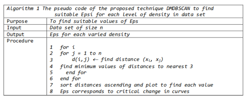
2023-01-11Parameters are an important aspect of any data mining task since they have a specific impact on the algorithm’s behavior. DBSCAN (Density-Based Spatial Clustering of Applications with Noise), a popular unsupervised machine learning technique for detecting clusters with varying shapes in a dataset, requires the user to specify two crucial parameters: epsilon (ε) and MinPts. These parameters must be set by the user to ensure the algorithm’s effectiveness.
This post will focus on estimating DBSCAN’s two parameters:
- Minimum samples (“MinPts”): the fewest number of points required to form a cluster
- ε (epsilon or “eps”): the maximum distance two points can be from one another while still belonging to the same cluster
Ideally, the value of ε is given by the problem to solve (e.g. a physical distance), and MinPts is then the desired minimum cluster size. The corresponding arguments for these parameters in the Scikit-Learn DBSCAN interface are eps and min_samples, respectively. Here is a general overview of selecting these parameters:
- MinPts: To derive the minimum value for MinPts, a rule of thumb is to set it to be greater than or equal to the number of dimensions D in the data set, i.e., MinPts ≥ D + 1. A low value of MinPts, such as 1, is not meaningful because it results in each point forming its own cluster. If MinPts≤ 2, the result will be similar to hierarchical clustering with the single link metric, where the dendrogram is cut at height ε. Therefore, MinPts must be at least 3. However, larger values are usually better for data sets with noise as they lead to more significant clusters. A value of MinPts = 2·D is a good rule of thumb, but larger values may be necessary for large or noisy data sets or those containing many duplicates.
- epsilon (ε): To choose the value of ε, a k-distance graph is plotted by ordering the distance to the k=MinPts-1 nearest neighbor from the largest to the smallest value. Good values of ε are where the plot shows an “elbow”. If ε is too small, a large portion of the data will not be clustered. If ε is too high, clusters will merge, and most objects will be in the same cluster. Small values of ε are generally preferred, and only a small fraction of points should be within this distance of each other. Alternatively, an OPTICS plot can be used to select ε, and the OPTICS algorithm can cluster the data.
- Distance function: The choice of distance function is closely related to the choice of ε and has a significant impact on the results. To select an appropriate distance function, a reasonable measure of similarity must first be identified for the data set. There is no estimation for this parameter, but distance functions need to be chosen appropriately for the data set. For instance, the great-circle distance is often a good choice for geographic data.
Details of determining DBSCAN parameters
1) k-distance plot
In a clustering with MinPts = k, we expect that core pints and border points’ k-distance are within a certain range, while noise points can have much greater k-distance, thus we can observe a knee point in the k-distance plot. However, sometimes there may be no obvious knee, or there can be multiple knees, which makes it hard to decide.
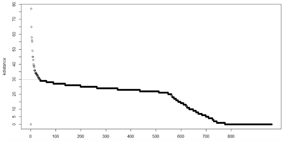
The method proposed here consists of computing the k-nearest neighbor distances in a matrix of points. The idea is to calculate, the average of the distances of every point to its k nearest neighbors. The value of k will be specified by the user and corresponds to MinPts. Next, these k-distances are plotted in ascending order. The aim is to determine the “knee”, which corresponds to the optimal epsilon parameter. A knee corresponds to a threshold where a sharp change occurs along the k-distance curve.
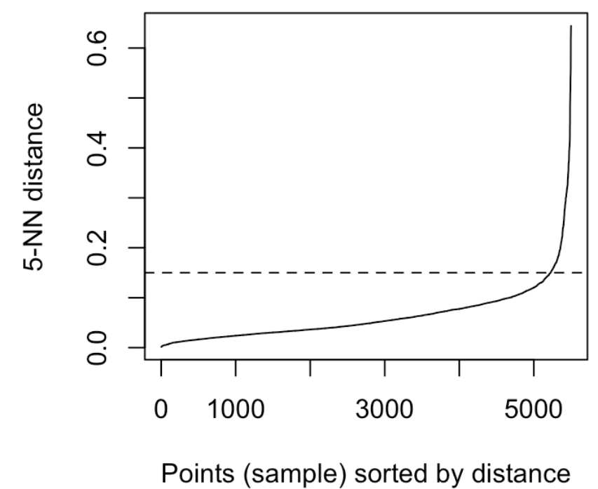
It can be seen that the optimal eps value is around a distance of 0.15.
2) DBSCAN extensions like OPTICS
OPTICS is a more generalized version of DBSCAN that substitutes the ε parameter with a maximum value, which mainly affects its performance. The MinPts parameter now denotes the minimum cluster size to be identified. Although the algorithm is much easier to parameterize than DBSCAN, its results are a bit more complex to use, as it typically generates a hierarchical clustering instead of the simple data partitioning produced by DBSCAN. Recently, one of the original authors of DBSCAN has revisited DBSCAN and OPTICS and introduced a revised version of hierarchical DBSCAN (HDBSCAN*) that eliminates the concept of border points. Only the core points now constitute the cluster.
OPTICS creates hierarchical clusters, we can extract significant flat clusters from them via visual inspection. An implementation of OPTICS is available in pyclustering. Additionally, one of the original authors of DBSCAN and OPTICS has proposed an automatic method to extract flat clusters that requires no human intervention. For more information, please refer to this paper.
3) Sensitivity Analysis
In essence, our aim is to select a radius that can cluster a higher number of truly regular points (i.e., points that are similar to other points) while also detecting more noise (i.e., outlier points). To achieve this, we can plot a percentage of regular points (i.e., points belonging to a cluster) versus epsilon analysis, wherein we set different epsilon values on the x-axis and their corresponding percentage of regular points on the y-axis. By analyzing the graph, we can identify a segment where the percentage of regular points is more sensitive to changes in the epsilon value. We can then select the upper bound epsilon value within this segment as our optimal parameter.
Some general rules for determining MinPts
The MinPts value is better to be set using domain knowledge and familiarity with the data set. Here are a few rules of thumb for selecting the MinPts value:
- The larger the data set, the larger the value of MinPts should be
- If the data set is noisier, choose a larger value of MinPts
- Generally, MinPts should be greater than or equal to the dimensionality of the data set
- For 2-dimensional data, use DBSCAN’s default value of MinPts = 4 (Ester et al., 1996).
- If your data has more than 2 dimensions, choose MinPts = 2*dim, where dim= the dimensions of your data set (Sander et al., 1998).
Python Example for selecting Epsilon (ε)
After selecting MinPts value, we can move on to determining ε. One technique to automatically determine the optimal ε value is described in this paper. This technique calculates the average distance between each point and its k nearest neighbors, where k is the MinPts value you selected. The average k-distances are then plotted in ascending order on a k-distance graph. We can find the optimal value for ε at the point of maximum curvature (i.e. where the graph has the greatest slope).
Suppose that we are working with a data set with 10 dimensions. Following the rules above, minimum_samples value should be at least 10. We can go with 20 (2*dim), as suggested in the literature.
After selecting MinPts value, we can use NearestNeighbors from Scikit-learn, documentation here, to calculate the average distance between each point and its n_neighbors. The one parameter we need to define is n_neighbors, which in this case is the value we choose for MinPts.
Step 1: Calculate the average distance between each point in the data set and its 20 nearest neighbors (my selected MinPts value).
from sklearn.neighbors import NearestNeighbors
from matplotlib import pyplot as plt

neighbors = NearestNeighbors(n_neighbors=20)
neighbors_fit = neighbors.fit(dataset)
distances, indices = neighbors_fit.kneighbors(dataset)
Step 2: Sort distance values by ascending value and plot.
distances = np.sort(distances, axis=0)
distances = distances[:,1]
plt.plot(distances)
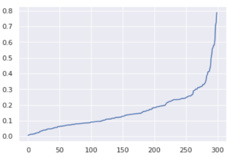
For this data set, the sorted distances produce a k-distance elbow plot that looks like this:
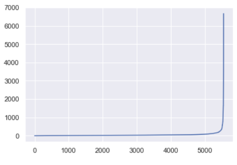
The ideal value for ε will be equal to the distance value at the “crook of the elbow”, or the point of maximum curvature. This point represents the optimization point where diminishing returns are no longer worth the additional cost. This concept of diminishing returns applies here because while increasing the number of clusters will always improve the fit of the model, it also increases the risk that overfitting will occur.
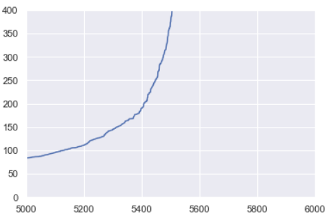
Zooming in on my k-distance plot, it looks like the optimal value for ε is around 225. We ended up looping through combinations of MinPts and ε values slightly above and below the values estimated here to find the model of best fit.
In layman’s terms, we find a suitable value for epsilon by calculating the distance to the nearest n points for each point, sorting, and plotting the results. Then we look to see where the change is most pronounced (think of the angle between your arm and forearm) and select that as epsilon.
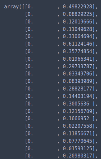
We can calculate the distance from each point to its closest neighbor using the NearestNeighbors. The point itself is included in n_neighbors. The kneighbors method returns two arrays, one which contains the distance to the closest n_neighbors points and the other which contains the index for each of those points.
nn_model = NearestNeighbors(n_neighbors=2)
nn_model.fit(X)
distances, indices = nn_model.kneighbors(X)
Next, we sort and plot the results.
distances = np.sort(distances, axis=0)
distances = distances[:,1]
plt.plot(distances)
The optimal value for epsilon will be found at the point of maximum curvature.
Reference:
4 Comments
Hi and thanks to sharing your work.
I have a question about the Min-samples. I have 2 attributes in my dataset, but this attributes are type=string, so I vettorized the attributes and I obtained a 1300 dimensions.
Min-samples must be = to 2+1 or 1300+1.
Thanks for your support
Hi Marcella,
You should set the min_samples based on the final input of your features to your model, that’s 1300+1. However, you generally should be careful about the problem of curse of dimensionality if you transform your features to such a high dimensional space.
Merci beaucoup pour votre explication. J ai une question comment fait fonction l ‘algorithme DBSCAN sur 3 dimensions sur le logiciel R, aurez vous une idée?
درود بر تو سفیدیان =)