Labeling financial data for Machine Learning
2021-06-26Machine Learning Interview: Training Neural Networks
2021-07-02Introduction
One of the most basic analysis functions is grouping and aggregating data. In some cases, this level of analysis may be sufficient to answer business questions. In other instances, this activity might be the first step in a more complex data science analysis. In pandas, the groupby function can be combined with one or more aggregation functions to quickly and easily summarize data. This concept is deceptively simple and most new pandas users will understand this concept. However, they might be surprised at how useful complex aggregation functions can be for supporting sophisticated analysis.
In this complete guide, you’ll learn (with examples):
- What is a Pandas GroupBy (object)?
- How to create summary statistics for groups with aggregation functions.
- How to create like-indexed objects of statistics for groups with the transformation method.
- How to use the flexible yet less efficient apply function.
- How to use custom functions for multiple columns.
Pandas GroupBy Method
The Pandas .groupby() method works in a very similar way to the SQL GROUP BY statement. In fact, it’s designed to mirror its SQL counterpart and leverage its efficiencies and intuitiveness. Similar to the SQL GROUP BY statement, the Pandas method works by splitting our data, aggregating it in a given way (or ways), and re-combining the data in a meaningful way.
Because the .groupby() method works by first splitting the data, we can actually work with the groups directly. Similarly, because any aggregations are done following the splitting, we have full reign over how we aggregate the data. Pandas then handles how the data are combined in order to present a meaningful DataFrame.
What’s great about this is that it allows us to use the method in a variety of ways, especially in creative ways. Because of this, the method is a cornerstone to understanding how Pandas can be used to manipulate and analyze data. This tutorial’s length reflects that complexity and importance!
Pandas seems to provide a myriad of options to help you analyze and aggregate our data. Why would there be, what often seems to be, an overlapping method? The answer is that each method, such as using the .pivot(), .pivot_table(), .groupby() methods, provide a unique spin on how data are aggregated. They’re not simply repackaged, but rather represent helpful ways to accomplish different tasks.
- Syntax: DataFrame.groupby(by=None, axis=0, level=None, as_index=True, sort=True,group_keys=True, observed=False, dropna=True)
- Purpose: To split the data into groups having similar characteristics, apply a function to them, and return the results after combining them in a data structure.
- Parameters:
- by: mapping or function or label or list of labels (default:None). We use this to determine the groups that have similar characteristics.
- axis: 0 or 1 (default: 0). We can use this to specify the orientation along which the DataFrame is to be split.
- level: Int or string or array (default:None). It is used to specify the name of the level in case the DataFrame has multi-level indices.
- as_index: Boolean (default: True). It is used to specify if the index of the output data structure should be the same as the group labels or not. This parameter is relevant only for a DataFrame input.
- sort: Boolean (default: True). It is used to specify if the output should be sorted according to the group keys or not. It does not affect the order of the observations within each group.
- group_keys: Boolean (default: True). We can use to determine if the group keys are to be added or not.
- observed: Boolean (default: False). It is used to specify if only the categorical groups are to be displayed or not. This parameter is applicable only if there is at least one categorical group.
- dropna: Boolean (default:True). It is used to specify if the NA values will be dropped from the group keys before returning the output or not. By default,they are dropped while making the groups.
- Returns: A groupby object containing the details of the groups formed in pandas.
Usage of pandas groupby: A basic example
Create a simple dataframe as shown below with details of employees of different departments
# Create DataFrame
import pandas as pd

# Create the data of the DataFrame as a dictionary
data_df = {'Name': ['Asha', 'Harsh', 'Sourav', 'Riya', 'Hritik',
                    'Shivansh', 'Rohan', 'Akash', 'Soumya', 'Kartik'],

           'Department': ['Administration', 'Marketing', 'Technical', 'Technical', 'Marketing',
                          'Administration', 'Technical', 'Marketing', 'Technical', 'Administration'],

           'Employment Type': ['Full-time Employee', 'Intern', 'Intern', 'Part-time Employee', 'Part-time Employee',
                               'Full-time Employee', 'Full-time Employee', 'Intern', 'Intern', 'Full-time Employee'],

           'Salary': [120000, 50000, 70000, 70000, 55000,
                      120000, 125000, 60000, 50000, 120000],

           'Years of Experience': [5, 1, 2, 3, 4,
                                   7, 6, 2, 1, 6]}

# Create the DataFrame
df = pd.DataFrame(data_df)
df
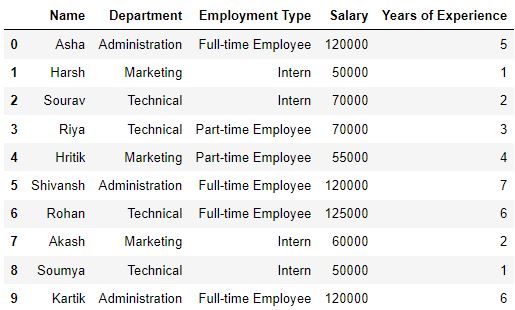
There are so many ways to create dataframes, if you don’t want to do it hard-coded like above.
Now, use groupby function to group the data as per the ‘Department’ type as shown below.
# Use pandas groupby to group rows by department and get only employees of technical department
df_grouped = df.groupby('Department')

df_grouped.get_group('Technical')

Let us say you want to find the average salary of different departments, then take the ‘Salary’ column from the grouped df and take the mean.
# Group by department and find average salary of each group
df.groupby('Department')['Salary'].mean()
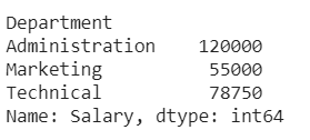
This is a common way of using the function. Now, let us dwell in depth on all the different ways possible.
The process of grouping the data
The process of grouping the data can be broken down into three steps:
- Splitting: Identity what column you want to do `groupby`. This is easily done using the
groupbymethod. - Applying: Apply the function or perform the operation for each group
- Combining: After applying the function, the results will be collected in one object.
Using a single key of groupby function in pandas
You can form groups using the groupby function using a single key (a ‘key’ is a column in the dataframe here) in pandas. The key can be a mapping, function, or the name of a column in a pandas DataFrame. In this case, the groupby key is a column named “Department”.
# Separate the rows into groups that have the same department
groups = df.groupby(by='Department')
You can view the different aspects of the output groups using multiple methods. You can use the groups method to view the index labels of the rows that have the same group key value. The output will be a dictionary where the keys of the dictionary are the group keys and the values of each key will be row index labels that have the same group key value.
# View the indices of the rows which are in the same group
print(groups.groups)
#> {'Administration': [0, 5, 9], 'Marketing': [1, 4, 7], 'Technical': [2, 3, 6, 8]}
As you can see, row indices 0, 5, and 9 have the group key value ‘Administration’, hence they have been grouped together.
Row indices 1, 4, 7 and 2, 3, 6, and 8 have been grouped together as they have their common values: ‘Marketing’ and ‘Technical’ respectively.
Using multiple keys in groupby function in pandas
You can also use several keys for making groups in pandas using the groupby function of pandas by passing the list of keys to the by parameter.
# Separate the rows into groups that have the same Department and Employment Type
groups = df.groupby(by=['Department', 'Employment Type'])
View the groups using the groups method.
# View the indices of the rows which are in the same group
groups.groups

# {('Administration', 'Full-time Employee'): [0, 5, 9], ('Marketing', 'Intern'): [1, 7], ('Marketing', 'Part-time Employee'): [4], ('Technical', 'Full-time Employee'): [6], ('Technical', 'Intern'): [2, 8], ('Technical', 'Part-time Employee'): [3]}
Iterating through the groups
You can use a ‘for’ loop to see the common group key value of each group as well as the rows of the pandas DataFrame which are a part of the same group.
# Separate the rows into groups that have the same department
groups = df.groupby(by='Department')

# View the name and the details of each group
for name, dept in groups:
    print(name)
    print(dept)
    print('\n')
Administration
       Name      Department     Employment Type  Salary  Years of Experience
0      Asha  Administration  Full-time Employee  120000                    5
5  Shivansh  Administration  Full-time Employee  120000                    7
9    Kartik  Administration  Full-time Employee  120000                    6


Marketing
     Name Department     Employment Type  Salary  Years of Experience
1   Harsh  Marketing              Intern   50000                    1
4  Hritik  Marketing  Part-time Employee   55000                    4
7   Akash  Marketing              Intern   60000                    2


Technical
     Name Department     Employment Type  Salary  Years of Experience
2  Sourav  Technical              Intern   70000                    2
3    Riya  Technical  Part-time Employee   70000                    3
6   Rohan  Technical  Full-time Employee  125000                    6
8  Soumya  Technical              Intern   50000                    1
Selecting a group
You can access the observations of that group by passing the group key value of a particular group to the get_group method,
# Separate the rows into groups that have the same department
groups = df.groupby('Department')

# View only that group whose group key value is 'Technical'
print(groups.get_group('Technical'))
     Name Department     Employment Type  Salary  Years of Experience
2  Sourav  Technical              Intern   70000                    2
3    Riya  Technical  Part-time Employee   70000                    3
6   Rohan  Technical  Full-time Employee  125000                    6
8  Soumya  Technical              Intern   50000                    1
Applying functions to a group
There are many functions that you can apply to the groups to get a statistical summary of the groups, transform the observations of the groups, or filter the groups based on certain criteria.
We can classify the functions broadly into three categories:
- Aggregation: These functions are used to compute different statistical values of the groups which can be useful for inferring insights about the trends or the pattern of observations present in the groups.
- Transformation: These functions are used to make certain changes and adjustments to the observations of the group.
- Filtration: These functions are used for subsetting the groups based on certain criteria.
1. Aggregation
There are several aggregation functions that you can apply to the groups such as ‘sum’ to get the sum of numeric features of a group, ‘count’ to get the number of occurrences of each group, or ‘mean’ to get the arithmetic mean of the numeric features of a group.
Use the aggregate method to apply the aggregation functions.
Example 1
# Separate the rows into groups that have the same department
groups = df.groupby(['Department'])

# View the sum of the numeric features of each group
groups.aggregate('sum')
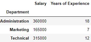
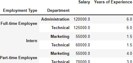
You can also apply aggregate functions on multiple keys by first making the groups with the keys and then passing the aggregation function to the method of the groups. The keys passed form a multilevel index of the data structure which contains the output.
Example 2
# Separate the rows into groups that have the same department nad employment type
groups = df.groupby(['Employment Type', 'Department'])

# View the average of the numeric features of each group
groups.aggregate('mean')
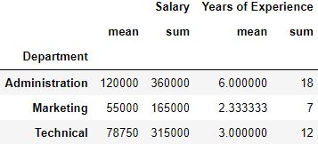
Applying multiple functions
By passing a list of functions to the aggregate method, you can view multiple statistical values of a group at a glance.
# Separate the rows into groups that have the same department
groups = df.groupby('Department')

# View the sum and the average of the numeric features of each group
groups.aggregate(['mean', 'sum'])
Applying different functions to different keys
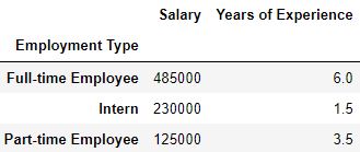
It is not necessary to apply the same aggregation function on all the keys. You can also apply different functions on different group keys by using a dictionary. The keys of the dictionary will be group keys and the values of the keys will be the function to be applied to them.
# Separate the rows into groups that have the same employment type
groups = df.groupby(['Employment Type'])

# Compute the sum on the salary feature and the mean on the Years of Experience feature of the groups
groups.aggregate({'Salary': 'sum', 'Years of Experience': 'mean'})
2. Transformation
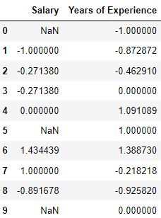
The transformation functions are used for making changes to the observations of each group. They can be used to apply important techniques such as standardization for scaling the observations of the group. Use the transformation method to apply the transformation functions.
Note that the transformation functions:
- It will return an output with the same size as the group chunk. Else, we will be able to broadcast the output to the same size as the group chunk.
- Operate on a column-to-column basis.
- We can’t use this for inplace operations. The groups formed must be considered to be immutable and applying transformation functions over them can yield unexpected results.
# Separate the rows into groups that have the same department
groups = df.groupby('Department')[["Salary", "Years of Experience"]]

# Define the transformation function to be applied
fun = lambda x: (x - x.mean())/x.std()

# Transform the groups
groups.transform(fun)
3. Filtration
If a data point or observation does not fulfill certain criteria, we can filter them. We use the filter method to apply the filtration functions.
# Separate the rows of the DataFrame into groups which have the same salary
groups = df.groupby('Salary')

# Filter out the groups whose average salary is less than 100000
groups.filter(lambda x: x['Salary'].mean() > 100000)

Other useful functions
Let’s look at a few more methods and functions available in the groups
The first method
We use this method to view the first observation of each group.
# Separate the rows into groups that have the same department
groups = df.groupby('Department')

# View the first observation of each group
groups.first()

The describe method
We use this method to display the statistical summary of the groups. It is similar to the .describe() method of the pandas DataFrames.
# Separate the rows into groups that have the same department
groups = df.groupby('Department')

# View the statistical summary of the groups
groups.describe()

The size method
This method shows the number of observations present in each group
# Separate the rows into groups that have the same department
groups = df.groupby('Department')

# View the number of observations present in each group
groups.size()
Department
Administration    3
Marketing         3
Technical         4
dtype: int64
The nunique method
This method shows the number of unique observations in each feature of the groups.
# Separate the rows into groups that have the same department
groups = df.groupby('Department')

# View the number of unique observations in each feature of the groups
groups.nunique()

Renaming columns
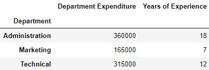
After applying a function, you can also rename the features of the groups by using the rename method to make them more descriptive.
This method requires a dictionary in which the keys are the original column names and the values are the new column names that will replace the original names.
# Separate the rows into groups that have the same department
groups = df.groupby('Department')

# Change the column name 'Salary' to 'Department Expenditure'
groups.aggregate('sum').rename(columns={'Salary': 'Department Expenditure'})
Practical Tips
- When you pass multiple group keys, only those rows whose group key values match with each other for all the group keys will be added to a group.
- Set the sort parameter as False for faster code execution.
- You can chain the steps of grouping and applying a function to reduce the lines of code.
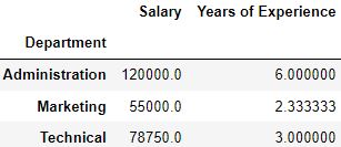
# Separate the rows into groups that have the same department and view the mean of the numeric features of the groups
df.groupby('Department').mean()
# Pass the Department feature first and then Employment Type
print(df.groupby(by=['Department', 'Employment Type']).mean())

print('\n')
# Pass the Department feature first and then Employment Type
print(df.groupby(by=['Employment Type', 'Department']).mean())
                                     Salary  Years of Experience
Department     Employment Type
Administration Full-time Employee  120000.0                  6.0
Marketing      Intern               55000.0                  1.5
               Part-time Employee   55000.0                  4.0
Technical      Full-time Employee  125000.0                  6.0
               Intern               60000.0                  1.5
               Part-time Employee   70000.0                  3.0


                                     Salary  Years of Experience
Employment Type    Department
Full-time Employee Administration  120000.0                  6.0
                   Technical       125000.0                  6.0
Intern             Marketing        55000.0                  1.5
                   Technical        60000.0                  1.5
Part-time Employee Marketing        55000.0                  4.0
                   Technical        70000.0                  3.0
More details about GroupBy
Let’s load a sample Pandas DataFrame.
# Loading a Sample Pandas DataFrame
import pandas as pd
df = pd.read_csv('https://raw.githubusercontent.com/datagy/data/main/sales.csv', parse_dates=['date'])
print(df.head())

# Returns:
#         date  gender      region  sales
# 0 2022-08-22    Male  North-West  20381
# 1 2022-03-05    Male  North-East  14495
# 2 2022-02-09    Male  North-East  13510
# 3 2022-06-22    Male  North-East  15983
# 4 2022-08-10  Female  North-West  15007
By printing out the first five rows using the .head() method, we can get a bit of insight into our data. We can see that we have a date column that contains the date of a transaction. We have string-type columns covering the gender and the region of our salesperson. Finally, we have an integer column, sales, representing the total sales value.
Understanding Pandas GroupBy Objects
Let’s take a first look at the Pandas .groupby() method. We can create a GroupBy object by applying the method to our DataFrame and passing in either a column or a list of columns. Let’s see what this looks like – we’ll create a GroupBy object and print it out:
# Creating a Pandas GroupBy Object
print(df.groupby('region'))

# Returns: <pandas.core.groupby.generic.DataFrameGroupBy object at 0x7fb78815a4f0>
We can see that this returned an object of type DataFrameGroupBy. Because it’s an object, we can explore some of its attributes.
Pandas GroupBy Attributes
For example, these objects come with an attribute, .ngroups, which holds the number of groups available in that grouping:
# Counting the Groups in a Pandas GroupBy Object
print(df.groupby('region').ngroups)

# Returns: 3
We can see that our object has 3 groups. Similarly, we can use the .groups attribute to gain insight into the specifics of the resulting groups. The output of this attribute is a dictionary-like object, which contains our groups as keys. The values of these keys are actually the indices of the rows belonging to that group!
# Accessing the Groups in a GroupBy object
print(df.groupby('region').groups)

# Returns: (truncated)
# {'North-East': [1, 2, 3, ...], 'North-West': [0, 4, 7, ...], 'South': [5, 6, 8, ...]}
If we only wanted to see the group names of our GroupBy object, we could simply return only the keys of this dictionary.
# Accessing only Group Names of a GroupBy Object
print(df.groupby('region').groups.keys())

# Returns: dict_keys(['North-East', 'North-West', 'South'])
We can see how useful this method already is! It allows us to group our data in a meaningful way.
Selecting a Pandas GroupBy Group
We can also select particular all the records belonging to a particular group. This can be useful when you want to see the data of each group. In order to do this, we can apply the .get_group() method and passing in the group’s name that we want to select. Let’s try and select the 'South' region from our GroupBy object:
# Selecting a Pandas GroupBy Group
print(df.groupby('region').get_group('South'))

# Returns:
#           date  gender region  sales
# 5   2022-09-06    Male  South  21792
# 6   2022-08-21    Male  South  20113
# 8   2022-11-22    Male  South  14594
# 9   2022-01-16  Female  South  24114
# 10  2022-12-21    Male  South  35154
# ..         ...     ...    ...    ...
# 972 2022-06-09    Male  South  22254
# 979 2022-11-24  Female  South  25591
# 981 2022-12-05    Male  South  34334
# 985 2022-12-01  Female  South  21282
# 994 2022-09-29    Male  South  21255

# [331 rows x 4 columns]
This can be quite helpful if you want to gain a bit of insight into the data. Similarly, it gives you insight into how the .groupby() method is actually used in terms of aggregating data. In the following section, you’ll learn how the Pandas groupby method works by using the split, apply, and combine methodology.
Understanding Pandas GroupBy Split-Apply-Combine
The Pandas groupby method uses a process known as split, apply, and combine to provide useful aggregations or modifications to your DataFrame. This process works just as its called:
- Splitting the data into groups based on some criteria
- Applying a function to each group independently
- Combing the results into an appropriate data structure
In the section above, when you applied the .groupby() method and passed in a column, you already completed the first step! You were able to split the data into relevant groups, based on the criteria you passed.
The reason for applying this method is to break a big data analysis problem into manageable parts. This allows you to perform operations on the individual parts and put them back together. While the apply and combine steps occur separately, Pandas abstracts this and makes it appear as though it was a single step.
Using Split-Apply-Combine Without GroupBy
Before we dive into how the .groupby() method works, let’s take a look at how we can replicate it without the use of the function. The benefit of this approach is that we can easily understand each step of the process.
- Splitting the data: Let’s begin by splitting the data – we can loop over each unique value in the DataFrame, splitting the data by the
'region'column. - Applying an aggregation function: From there, we can select the rows from the DataFrame that meet the condition and apply a function to it.
- Combining the Data: Finally, we can create a dictionary and add data to it and turn it back into a Pandas DataFrame.
# Replicating split-apply-combine Without GroupBy

# Create a Container Dictionary
averages = {}

# Split the data into different regions
for region in df['region'].unique():
    tempdf = df[df['region'] == region]

    # Apply an aggregation function
    average = tempdf['sales'].mean()

    # Combine the data into a DataFrame
    averages[region] = [average]

aggregate_df = pd.DataFrame.from_dict(averages, orient='index', columns=['Average Sales'])
print(aggregate_df)

# Returns:
#             Average Sales
# North-West   15257.732919
# North-East   17386.072046
# South        24466.864048
This is a lot of code to write for a simple aggregation! Thankfully, the Pandas groupby method makes this much, much easier. In the next section, you’ll learn how to simplify this process tremendously.
Aggregating Data with Pandas GroupBy
In this section, you’ll learn how to use the Pandas groupby method to aggregate data in different ways. We’ll try and recreate the same result as you learned about above in order to see how much simpler the process actually is! Let’s take a look at what the code looks like and then break down how it works:
# Aggregating Data with Pandas .groupby()
averages = df.groupby('region')['sales'].mean()
print(averages)

# Returns:
# region
# North-East    17386.072046
# North-West    15257.732919
# South         24466.864048
# Name: sales, dtype: float64
Take a look at the code! We were able to reduce six lines of code into a single line! Let’s break this down element by element:
df.groupby('region')is familiar to you by now. It splits the data into different groups, based on theregioncolumn['sales']selects only that column from the groupings.mean()applies the mean method to the column in each group- The data are combined into the resulting DataFrame,
averages
Let’s take a look at the entire process a little more visually. In order to make it easier to understand visually, let’s only look at the first seven records of the DataFrame:
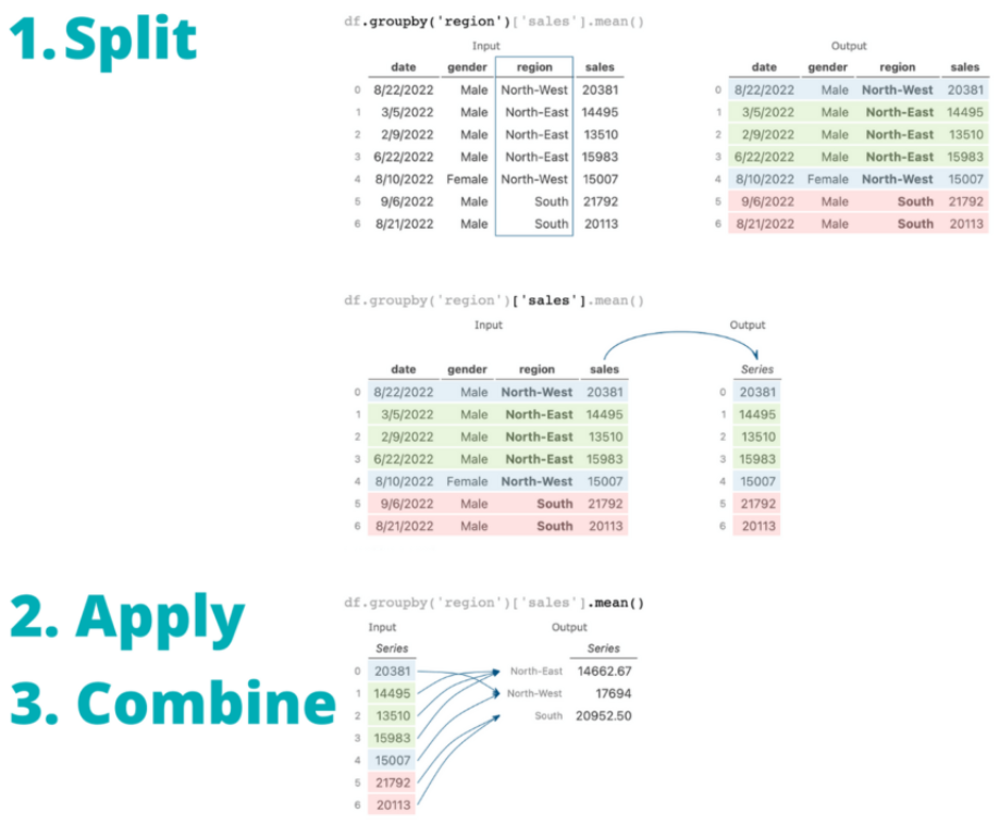
.groupby()In the image above, you can see how the data is first split into groups and a column is selected, then an aggregation method is applied and the resulting data are combined.
Other Aggregations with Pandas GroupBy
Now that you understand how the split-apply-combine procedure works, let’s take a look at some other aggregations that work in Pandas. The table below provides an overview of the different available aggregation functions:
| Aggregation Method | Description |
|---|---|
.count() | The number of non-null records |
.sum() | The sum of the values |
.mean() | The arithmetic mean of the values |
.median() | The median of the values |
.min() | The minimum value of the group |
.max() | The maximum value of the group |
.mode() | The most frequent value in the group |
.std() | The standard deviation of the group |
.var() | The variance of the group |
For example, if we wanted to calculate the standard deviation of each group, we could simply write:
# Calculating the Standard Deviation of Each Group's Sales
standard_deviations = df.groupby('region')['sales'].std()
print(standard_deviations)

# Returns:
# region
# North-East    2032.541552
# North-West    3621.456493
# South         5253.702513
# Name: sales, dtype: float64
Applying Multiple Aggregations Using Pandas GroupBy
Pandas also comes with an additional method, .agg(), which allows us to apply multiple aggregations in the .groupby() method. The method allows us to pass in a list of callables (i.e., the function part without the parentheses). Let’s see how we can apply some of the functions that come with the numpy library to aggregate our data.
# Applying Multiple Aggregations with .agg()
import numpy as np
aggs = df.groupby('region')['sales'].agg([np.mean, np.std, np.var])
print(aggs)

# Returns:
#                     mean          std           var
# region
# North-East  17386.072046  2032.541552  4.131225e+06
# North-West  15257.732919  3621.456493  1.311495e+07
# South       24466.864048  5253.702513  2.760139e+07
Using the .agg() method allows us to easily generate summary statistics based on our different groups. Without this, we would need to apply the .groupby() method three times but here we were able to reduce it down to a single method call!
Transforming Data with Pandas GroupBy
Another incredibly helpful way you can leverage the Pandas groupby method is to transform your data. What does this mean? By transforming your data, you perform some operations specific to that group. This can include, for example, standardizing the data based only on that group using a z-score or dealing with missing data by imputing a value based on that group.
What makes the transformation operation different from both aggregation and filtering using .groupby() is that the resulting DataFrame will be the same dimensions as the original data. While this can be true for aggregating and filtering data, it is always true for transforming data.
The .transform() method will return a single value for each record in the original dataset. Because of this, the shape is guaranteed to result in the same size.
Using .transform In GroupBy
Let’s take a look at an example of transforming data in a Pandas DataFrame. In this example, we’ll calculate the percentage of each region’s total sales represented by each sale. To do this, we can apply the .transform() method to the GroupBy object. We can pass in the 'sum' callable to return the sum for the entire group onto each row. Finally, we divide the original 'sales' column by that sum.
Let’s see what this code looks like:
# Calculating percentage of region's sales
df['Percent Of Region Sales'] = df['sales'] / df.groupby('region')['sales'].transform('sum')
print(df.head())

# Returns:
#         date  gender      region  sales  Percent Of Region Sales
# 0 2022-08-22    Male  North-West  20381                 0.004148
# 1 2022-03-05    Male  North-East  14495                 0.002403
# 2 2022-02-09    Male  North-East  13510                 0.002239
# 3 2022-06-22    Male  North-East  15983                 0.002649
# 4 2022-08-10  Female  North-West  15007                 0.003055
In the resulting DataFrame, we can see how much each sale accounted for out of the region’s total.
Transforming Data without .transform
While in the previous section, you transformed the data using the .transform() function, we can also apply a function that will return a single value without aggregating. As an example, let’s apply the .rank() method to our grouping. This will allow us to, well, rank our values in each group. Rather than using the .transform() method, we’ll apply the .rank() method directly:
# Transforming a DataFrame with GroupBy
df['ranked'] = df.groupby('region')['sales'].rank(ascending=False)
print(df.sort_values(by='sales', ascending=False).head())

# Returns:
#           date  gender region  sales  ranked
# 61  2022-02-22  Female  South  43775     1.0
# 673 2022-04-19    Male  South  37878     2.0
# 111 2022-10-31  Female  South  36444     3.0
# 892 2022-09-05    Male  South  35723     4.0
# 136 2022-02-27    Male  South  35485     5.0
In this case, the .groupby() method returns a Pandas Series of the same length as the original DataFrame. Because of this, we can simply assign the Series to a new column.
Filtering Data with Pandas GroupBy
A great way to make use of the .groupby() method is to filter a DataFrame. This approach works quite differently from a normal filter since you can apply the filtering method based on some aggregation of a group’s values. For example, we can filter our DataFrame to remove rows where the group’s average sale price is less than 20,000.
# Filtering Rows Where the Group's Average Sale Price is Less Than 20,000
df = df.groupby('region').filter(lambda x: x['sales'].mean() < 20000)
print(df.head())

# Returns:
#         date  gender      region  sales
# 0 2022-08-22    Male  North-West  20381
# 1 2022-03-05    Male  North-East  14495
# 2 2022-02-09    Male  North-East  13510
# 3 2022-06-22    Male  North-East  15983
# 4 2022-08-10  Female  North-West  15007
Let’s break down how this works:
- We group our data by the
'region'column - We apply the
.filter()method to filter based on a lambda function that we pass in - The lambda function evaluates whether the average value found in the group for the
'sales'column is less than 20,000
This approach saves us the trouble of first determining the average value for each group and then filtering these values out. In this example, the approach may seem a bit unnecessary. However, it opens up massive potential when working with smaller groups.
Grouping a Pandas DataFrame by Multiple Columns
We can extend the functionality of the Pandas .groupby() method even further by grouping our data by multiple columns. So far, you’ve grouped the DataFrame only by a single column, by passing in a string representing the column. However, you can also pass in a list of strings that represent the different columns. By doing this, we can split our data even further.
Let’s calculate the sum of all sales broken out by 'region' and by 'gender' by writing the code below:
# Grouping Data by Multiple Columns
sums = df.groupby(['region', 'gender']).sum()
print(sums.head())

# Returns:
#                      sales
# region     gender
# North-East Female  3051132
#            Male    2981835
# North-West Female  2455899
#            Male    2457091
# South      Female  4135688
What’s more, is that all the methods that we previously covered are possible in this regard as well. For example, we could apply the .rank() function here again and identify the top sales in each region-gender combination:
# Ranking Sales by Region and by Gender
df['rank'] = df.groupby(['region', 'gender'])['sales'].rank(ascending=False)
print(df.head())

# Returns:
#         date  gender      region  sales   rank
# 0 2022-08-22    Male  North-West  20381   11.0
# 1 2022-03-05    Male  North-East  14495  154.0
# 2 2022-02-09    Male  North-East  13510  168.0
# 3 2022-06-22    Male  North-East  15983  138.0
# 4 2022-08-10  Female  North-West  15007   89.5
Using Custom Functions with Pandas GroupBy
Another excellent feature of the Pandas .groupby() method is that we can even apply our own functions. This allows us to define functions that are specific to the needs of our analysis. You’ve actually already seen this in the example to filter using the .groupby() method. We can either use an anonymous lambda function or we can first define a function and apply it.
Let’s take a look at how this can work. We can define a custom function that will return the range of a group by calculating the difference between the minimum and the maximum values. Let’s define this function and then apply it to our .groupby() method call:
# Using a User-Defined Function in a GroupBy Object
def group_range(x):
    return x.max() - x.min()

ranges = df.groupby(['region', 'gender'])['sales'].apply(group_range)
print(ranges)

# Returns:
# region      gender
# North-East  Female    10881
#             Male      10352
# North-West  Female    20410
#             Male      17469
# South       Female    30835
#             Male      27110
# Name: sales, dtype: int64
The group_range() function takes a single parameter, which in this case is the Series of our 'sales' groupings. We find the largest and smallest values and return the difference between the two. This can be helpful to see how different groups’ ranges differ.
More examples of Pandas GroupBy
In this section, you’ll learn some helpful use cases of the Pandas .groupby() method. The examples in this section are meant to represent more creative uses of the method. These examples are meant to spark creativity and open your eyes to different ways in which you can use the method.
Getting the First n Rows of a Pandas GroupBy
Let’s take a look at how you can return the five rows of each group into a resulting DataFrame. This can be particularly helpful when you want to get a sense of what the data might look like in each group. If it doesn’t matter how the data are sorted in the DataFrame, then you can simply pass in the .head() function to return any number of records from each group.
Let’s take a look at how to return two records from each group, where each group is defined by the region and gender:
# Return the first two records of each group
print(df.groupby(['region', 'gender']).head(2))

# Returns:
#          date  gender      region  sales
# 0  2022-08-22    Male  North-West  20381
# 1  2022-03-05    Male  North-East  14495
# 2  2022-02-09    Male  North-East  13510
# 4  2022-08-10  Female  North-West  15007
# 5  2022-09-06    Male       South  21792
# 6  2022-08-21    Male       South  20113
# 7  2022-07-08    Male  North-West  13650
# 9  2022-01-16  Female       South  24114
# 11 2022-04-30  Female  North-West  19631
# 12 2022-11-25  Female  North-East  18262
# 13 2022-08-14  Female  North-East  13733
# 20 2022-01-21  Female       South  32313
Getting the nth Largest Row of a Pandas GroupBy
In this example, you’ll learn how to select the nth largest value in a given group. For this, we can use the .nlargest() method which will return the largest value of position n. For example, if we wanted to return the second largest value in each group, we could simply pass in the value 2. Let’s see what this looks like:
# Getting the second largest value in each group
print(df.groupby(['region', 'gender'])['sales'].nlargest(2))

# Returns:
# region      gender
# North-East  Female  407    22545
#                     561    21933
#             Male    560    22361
#                     442    21951
# North-West  Female  758    26813
#                     46     24573
#             Male    844    23553
#                     576    23485
# South       Female  61     43775
#                     111    36444
#             Male    673    37878
#                     892    35723
# Name: sales, dtype: int64
Aggregating
An aggregation function is one that takes multiple individual values and returns a summary. In the majority of the cases, this summary is a single value. The most common aggregation functions are a simple average or summation of values. As of pandas 0.20, you may call an aggregation function on one or more columns of a DataFrame. Here’s a quick example of calculating the total and average fare using the Titanic dataset (loaded from seaborn):
import pandas as pd
import seaborn as sns

df = sns.load_dataset('titanic')

df['fare'].agg(['sum', 'mean'])

sum     28693.949300
mean       32.204208
Name: fare, dtype: float64
This simple concept is a necessary building block for more complex analysis. One area that needs to be discussed is that there are multiple ways to call an aggregation function. As shown above, you may pass a list of functions to apply to one or more columns of data. What if you want to perform the analysis on only a subset of columns? There are two other options for aggregations: using a dictionary or a named aggregation.
Here is a comparison of the three options:
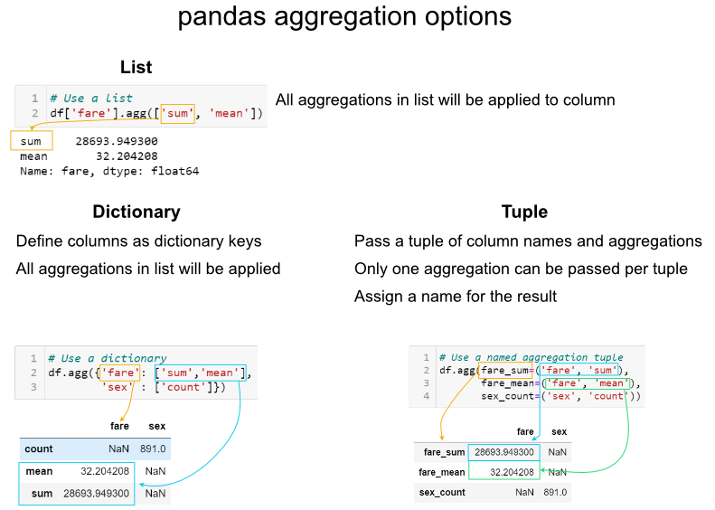
It is important to be aware of these options and know which one to use when. Generally, I prefer to use dictionaries for aggregations. The tuple approach is limited by only being able to apply one aggregation at a time to a specific column. If I need to rename columns, then I will use the rename function after the aggregations are complete. In some specific instances, the list approach is a useful shortcut. I will reiterate though, that I think the dictionary approach provides the most robust approach for the majority of situations.
Groupby Examples
Basic math
The most common built-in aggregation functions are basic math functions including sum, mean, median, minimum, maximum, standard deviation, variance, mean absolute deviation, and product.
We can apply all these functions to the fare while grouping by the embark_town :
agg_func_math = {
    'fare':
    ['sum', 'mean', 'median', 'min', 'max', 'std', 'var', 'mad', 'prod']
}
df.groupby(['embark_town']).agg(agg_func_math).round(2)

This is all relatively straightforward math. As an aside, I have not found a good usage for the prod function which computes the product of all the values in a group. For the sake of completeness, I am including it. One other useful shortcut is to use describe to run multiple built-in aggregations at one time:
agg_func_describe = {'fare': ['describe']}
df.groupby(['embark_town']).agg(agg_func_describe).round(2)

Counting
After basic math, counting is the next most common aggregation I perform on grouped data. In some ways, this can be a little more tricky than the basic math. Here are three examples of counting:
agg_func_count = {'embark_town': ['count', 'nunique', 'size']}
df.groupby(['deck']).agg(agg_func_count)

The major distinction to keep in mind is that count will not include NaN values whereas size will. Depending on the data set, this may or may not be a useful distinction. In addition, the nunique function will exclude NaN values in the unique counts. Keep reading for an example of how to include NaN in the unique value counts.
First and last
In this example, we can select the highest and lowest fare by embarked town. One important point to remember is that you must sort the data first if you want first and last to pick the max and min values.
agg_func_selection = {'fare': ['first', 'last']}
df.sort_values(by=['fare'],
            ascending=False).groupby(['embark_town'
                                        ]).agg(agg_func_selection)

In the example above, I would recommend using max and min but I am including first and last for the sake of completeness. In other applications (such as time series analysis) you may want to select the first and last values for further analysis. Another selection approach is to use idxmax and idxmin to select the index value that corresponds to the maximum or minimum value.
agg_func_max_min = {'fare': ['idxmax', 'idxmin']}
df.groupby(['embark_town']).agg(agg_func_max_min)

We can check the results:
df.loc[[258, 378]]

Here’s another shortcut trick you can use to see the rows with the max fare :
df.loc[df.groupby('class')['fare'].idxmax()]

The above example is one of those places where list-based aggregation is a useful shortcut.
Other libraries
You are not limited to the aggregation functions in pandas. For instance, you could use stats functions from scipy or numpy. Here is an example of calculating the mode and skew of the fare data.
from scipy.stats import skew, mode
agg_func_stats = {'fare': [skew, mode, pd.Series.mode]}
df.groupby(['embark_town']).agg(agg_func_stats)

The mode results are interesting. The scipy.stats mode function returns the most frequent value as well as the count of occurrences. If you just want the most frequent value, use pd.Series.mode. The key point is that you can use any function you want as long as it knows how to interpret the array of pandas values and returns a single value.
Working with text
When working with text, the counting functions will work as expected. You can also use scipy’s mode function on text data. One interesting application is that if you a have a small number of distinct values, you can use python’s set function to display the full list of unique values.
This summary of the class and deck shows how this approach can be useful for some data sets.
agg_func_text = {'deck': [ 'nunique', mode, set]}
df.groupby(['class']).agg(agg_func_text)

Custom functions
The pandas standard aggregation functions and pre-built functions from the python ecosystem will meet many of your analysis needs. However, you will likely want to create your own custom aggregation functions. There are four methods for creating your own functions.
To illustrate the differences, let’s calculate the 25th percentile of the data using four approaches:
First, we can use a partial function:
from functools import partial
# Use partial
q_25 = partial(pd.Series.quantile, q=0.25)
q_25.__name__ = '25%'
Next, we define our own function (which is a small wrapper around quantile ):
# Define a function
def percentile_25(x):
    return x.quantile(.25)
We can define a lambda function and give it a name:
# Define a lambda function
lambda_25 = lambda x: x.quantile(.25)
lambda_25.__name__ = 'lambda_25%'
Or, define the lambda inline:
# Use a lambda function inline
agg_func = {
    'fare': [q_25, percentile_25, lambda_25, lambda x: x.quantile(.25)]
}

df.groupby(['embark_town']).agg(agg_func).round(2)

As you can see, the results are the same but the labels of the column are all a little different. This is an area of programmer preference but I encourage you to be familiar with the options since you will encounter most of these in online solutions.
Custom function examples
As shown above, there are multiple approaches to developing custom aggregation functions. I will go through a few specific useful examples to highlight how they are frequently used. In most cases, the functions are lightweight wrappers around built-in pandas functions. Part of the reason you need to do this is that there is no way to pass arguments to aggregations. Some examples should clarify this point.
If you want to count the number of null values, you could use this function:
def count_nulls(s):
    return s.size - s.count()
If you want to include NaN values in your unique counts, you need to pass dropna=False to the nunique function.
def unique_nan(s):
    return s.nunique(dropna=False)
Here is a summary of all the values together:
agg_func_custom_count = {
    'embark_town': ['count', 'nunique', 'size', unique_nan, count_nulls, set]
}
df.groupby(['deck']).agg(agg_func_custom_count)

If you want to calculate the 90th percentile, use quantile :
def percentile_90(x):
    return x.quantile(.9)
If you want to calculate a trimmed mean where the lowest 10th percent is excluded, use the scipy stats function trim_mean :
def trim_mean_10(x):
    return trim_mean(x, 0.1)
If you want the largest value, regardless of the sort order (see notes above about first and last :
def largest(x):
    return x.nlargest(1)
This is equivalent to max but I will show another example of nlargest below to highlight the difference.
def sparkline_str(x):
    bins=np.histogram(x)[0]
    sl = ''.join(sparklines(bins))
    return sl
Here they are all put together:
agg_func_largest = {
    'fare': [percentile_90, trim_mean_10, largest, sparkline_str]
}
df.groupby(['class', 'embark_town']).agg(agg_func_largest)

The nlargest and nsmallest functions can be useful for summarizing the data in various scenarios. Here is the code to show the total fares for the top 10 and bottom 10 individuals:
def top_10_sum(x):
    return x.nlargest(10).sum()

def bottom_10_sum(x):
    return x.nsmallest(10).sum()

agg_func_top_bottom_sum = {
    'fare': [top_10_sum, bottom_10_sum]
}
df.groupby('class').agg(agg_func_top_bottom_sum)

Using this approach can be useful when applying the Pareto principle to your own data.
Custom functions with multiple columns
If you have a scenario where you want to run multiple aggregations across columns, then you may want to use the groupby combined with apply as described in this stack overflow answer. Using this method, you will have access to all of the columns of the data and can choose the appropriate aggregation approach to build up your resulting DataFrame (including the column labels):
def summary(x):
    result = {
        'fare_sum': x['fare'].sum(),
        'fare_mean': x['fare'].mean(),
        'fare_range': x['fare'].max() - x['fare'].min()
    }
    return pd.Series(result).round(0)

df.groupby(['class']).apply(summary)

Using apply with groupy gives maximum flexibility over all aspects of the results. However, there is a downside. The apply function is slow so this approach should be used sparingly.
Working with group objects
Once you group and aggregate the data, you can do additional calculations on the grouped objects. For the first example, we can figure out what percentage of the total fares sold can be attributed to each embark_town and class combination. We use assign and a lambda function to add a pct_total column:
df.groupby(['embark_town', 'class']).agg({
    'fare': 'sum'
}).assign(pct_total=lambda x: x / x.sum())

One important thing to keep in mind is that you can actually do this more simply using a pd.crosstab.
pd.crosstab(df['embark_town'],
            df['class'],
            values=df['fare'],
            aggfunc='sum',
            normalize=True)

While we are talking about crosstab , a useful concept to keep in mind is that agg functions can be combined with pivot tables too.
Here’s a quick example:
pd.pivot_table(data=df,
            index=['embark_town'],
            columns=['class'],
            aggfunc=agg_func_top_bottom_sum)

Sometimes you will need to do multiple groupby’s to answer your question. For instance, if we wanted to see a cumulative total of the fares, we can group and aggregate by town and class then group the resulting object and calculate a cumulative sum:
fare_group = df.groupby(['embark_town', 'class']).agg({'fare': 'sum'})
fare_group.groupby(level=0).cumsum()

This may be a little tricky to understand. Here’s a summary of what we are doing:

Here’s another example where we want to summarize daily sales data and convert it to a cumulative daily and quarterly view. In the first example, we want to include the total daily sales as well as the cumulative quarter amount:
sales = pd.read_excel('https://github.com/chris1610/pbpython/blob/master/data/2018_Sales_Total_v2.xlsx?raw=True')

daily_sales = sales.groupby([pd.Grouper(key='date', freq='D')
                            ]).agg(daily_sales=('ext price',
                                                'sum')).reset_index()
daily_sales['quarter_sales'] = daily_sales.groupby(
    pd.Grouper(key='date', freq='Q')).agg({'daily_sales': 'cumsum'})
To understand this, you need to look at the quarter boundary (end of March through the start of April) to get a good sense of what is going on.

If you want to just get a cumulative quarterly total, you can chain multiple groupby functions. First, group the daily results, then group those results by quarter and use a cumulative sum:
sales.groupby([pd.Grouper(key='date', freq='D')
            ]).agg(daily_sales=('ext price', 'sum')).groupby(
                pd.Grouper(freq='Q')).agg({
                    'daily_sales': 'cumsum'
                }).rename(columns={'daily_sales': 'quarterly_sales'})

In this example, I included the named aggregation approach to rename the variable to clarify that it is now daily sales. I then group again and use the cumulative sum to get a running sum for the quarter. Finally, I rename the column to quarterly sales. Admittedly this is a bit tricky to understand. However, if you take it step by step and build out the function and inspect the results at each step, you will start to get the hang of it. Don’t be discouraged!
Flattening Hierarchical Column Indices
By default, pandas creates a hierarchical column index on the summary DataFrame. Here is what I am referring to:
df.groupby(['embark_town', 'class']).agg({'fare': ['sum', 'mean']}).round(0)

At some point in the analysis process, you will likely want to “flatten” the columns so that there is a single row of names. I have found that the following approach works best for me. I use the parameter as_index=False when grouping, then build a new collapsed column name. Here is the code:
multi_df = df.groupby(['embark_town', 'class'],
                    as_index=False).agg({'fare': ['sum', 'mean']})

multi_df.columns = [
'_'.join(col).rstrip('_') for col in multi_df.columns.values
]
Here is a picture showing what the flattened frame looks like:

I prefer to use _ as my separator but you could use other values. Just keep in mind that it will be easier for your subsequent analysis if the resulting column names do not have spaces.
Subtotals
One process that is not straightforward with grouping and aggregating in pandas is adding a subtotal. If you want to add subtotals, I recommend the sidetable package. Here is how you can summarize fares by class , embark_town and sex with a subtotal at each level as well as a grand total at the bottom:
import sidetable
df.groupby(['class', 'embark_town', 'sex']).agg({'fare': 'sum'}).stb.subtotal()
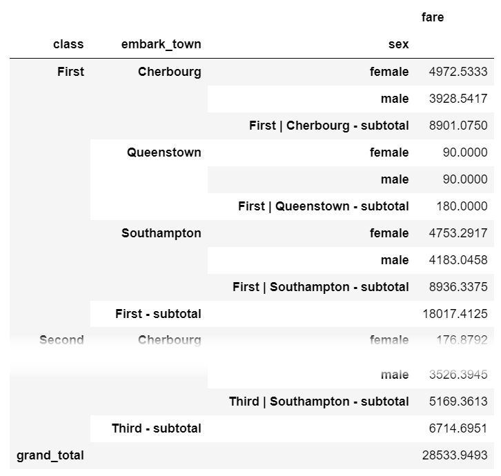
sidetable also allows customization of the subtotal levels and resulting labels. Refer to the package documentation for more examples of how sidetable can summarize your data.
Another case study: Hypothetical Sales Division
We are going to use data from a hypothetical sales division in this example. The data set consists, among other columns, of fictitious sales reps, order leads, the company the deal might close with, order values, and the date of the lead.
order_leads = pd.read_csv(
    'https://raw.githubusercontent.com/FBosler/Medium-Data-Exploration/master/order_leads.csv',
    parse_dates = [3]
)
sales_team = pd.read_csv(
    'https://raw.githubusercontent.com/FBosler/Medium-Data-Exploration/master/sales_team.csv',
    parse_dates = [3]
)
df = pd.merge(
  order_leads,
  sales_team,
  on=['Company Id','Company Name']
)
df = df.rename(
  columns={'Order Value':'Val','Converted':'Sale'}
)
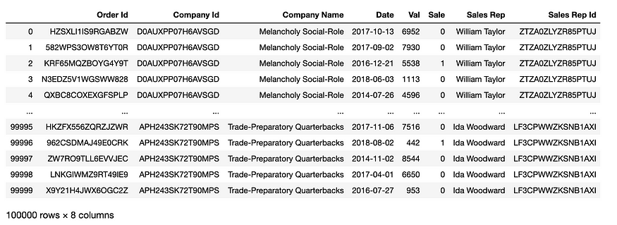
Groupby — Splitting the Data
The default approach of calling groupby is by explicitly providing a column name to split the dataset by. However, and this is less known, you can also pass a Series to groupby. The only restriction is that the series has the same length as the DataFrame. Being able to pass a series means that you can group by a processed version of a column, without having to create a new helper column for that.
Group by sales rep
First, let’s create a grouped DataFrame, i.e., split the dataset up.
grouped = df.groupby('Sales Rep')
grouped

# OUT:
<pandas.core.groupby.generic.DataFrameGroupBy object at 0x12464a160>

type(grouped)

# OUT:
pandas.core.groupby.generic.DataFrameGroupBy
We have now created a DataFrameGroupBy object. Let’s further investigate:
Show all groups
Calling groups on the grouped object returns the list of indices for every group (as every row can be uniquely identified via its index)
grouped.groups

# OUT:
{
'Aaron Hendrickson': Int64Index(
[25612, 25613, 25614, 25615, 25616, 25617, 25618, 25619, 25620, 25621,..., 25894, 25895, 25896, 25897, 25898, 25899, 25900, 25901, 25902, 25903], dtype='int64', length=292
),'Adam Sawyer': Int64Index(
[67140, 67141, 67142, 67143, 67144, 67145, 67146, 67147, 67148, 67149, ..., 67454, 67455, 67456, 67457, 67458, 67459, 67460, 67461, 67462, 67463], dtype='int64', length=324
),...'Yvonne Lindsey': Int64Index([20384, 20385, 20386, 20387, 20388, 20389, 20390, 20391, 20392, 20393, 20394, 20395, 20396, 20397, 20398, 20399, 20400, 20401, ... , 20447, 20448, 20449, 20450], dtype='int64', length=67)
}
Select a specific group
By calling get_group with the name of the group, we can return the respective subset of the data.
grouped.get_group('Aaron Hendrickson')

To demonstrate some advanced grouping functionalities, we will use the simplest version of the apply step (and count the rows in each group) via the size method. We do this so that we can focus on the groupby operations. We will go into much more detail regarding the apply methods in the next section.
Count rows in each group
grouped.size()

# OUT:
Sales Rep
Aaron Hendrickson    292
Adam Sawyer          324
Adele Kimmel         115
Adrian Daugherty     369
Adrianna Shelton      37
                    ...
Willie Lin            44
Willie Rau            95
Willie Sanchez       309
Yvonne Jones          74
Yvonne Lindsey        67
Length: 499, dtype: int64
Group by the first name of sales rep
The following is the first example where we group by a variation of one of the existing columns. I find this is a vast improvement over creating helper columns all the time. It just keeps the data cleaner. In this example, we use a string accessor to retrieve the first name.
df.groupby(
  df['Sales Rep'].str.split(' ').str[0]
).size()

# OUT:
Sales Rep
Aaron        292
Adam         324
Adele        115
Adrian       369
Adrianna      37
            ...
Wesley       144
Wilbert      213
William     1393 # Plenty of Williams
Willie       448
Yvonne       141
Length: 318, dtype: int64
Grouping by whether or not there is a “William” in the name of the rep
We saw that there seem to be a lot of Williams, lets’s group all sales reps who have William in their name together.
df.groupby(
  df['Sales Rep'].apply(lambda x: 'William' in x)
).size()

# OUT:
Sales Rep
False    97111
True      2889
dtype: int64
Group by random series (for illustrative purposes only)
This example is — admittedly — silly, but it illustrates the point that you can group by arbitrary series quite well.
df.groupby(
    pd.Series(np.random.choice(list('ABCDG'),len(df)))
).size()

# OUT:
A    19895
B    20114
C    19894
D    20108
G    19989
dtype: int64
Grouping by three evenly cut “Val” buckets
In the following example, we apply qcut to a numerical column first. qcut allocates the data equally into a fixed number of bins.
df.groupby(
  pd.qcut(
    x=df['Val'],
    q=3,
    labels=['low','mid','high']
  )
).size()

# OUT:
Val
low     33339
mid     33336
high    33325
dtype: int64
Grouping by custom-sized “Val” buckets
Like in the previous example, we allocate the data to buckets. This time, however, we also specify the bin boundaries.
df.groupby(
  pd.cut(
    df['Val'],
    [0,3000,5000,7000,10000]
  )
).size()

# OUT:
Val
(0, 3000]        29220
(3000, 5000]     19892
(5000, 7000]     20359
(7000, 10000]    30529
dtype: int64
pd.Grouper
pd.Grouper is important! This one took me way too long to learn, as it is incredibly helpful when working with time-series data.
Grouping by year
In the following example, we are going to use pd.Grouper(key=<INPUT COLUMN>, freq=<DESIRED FREQUENCY>) to group our data based on the specified frequency for the specified column. In our case, the frequency is 'Y' and the relevant column is 'Date'.
df.groupby(
  pd.Grouper(
    key='Date',
    freq='Y'
  )
).size()

# OUT:
Date
2014-12-31    19956
2015-12-31    20054
2016-12-31    20133
2017-12-31    20079
2018-12-31    19778
Freq: A-DEC, dtype: int64
Grouping by quarter or other frequencies
Instead of 'Y' we can use different standard frequencies like 'D','W','M', or 'Q'. For a list of less common usable frequencies, check out the documentation. I found'SM' for semi-month end frequency (15th and end of the month) to be an interesting one.
df.groupby(pd.Grouper(key='Date',freq='Q')).size()

#OUT:
Date
2014-03-31    4949
2014-06-30    4948
2014-09-30    4986
2014-12-31    5073
2015-03-31    4958
2015-06-30    4968
2015-09-30    5109
2015-12-31    5019
2016-03-31    5064
2016-06-30    4892
2016-09-30    5148
2016-12-31    5029
2017-03-31    4959
2017-06-30    5102
2017-09-30    5077
2017-12-31    4941
2018-03-31    4889
2018-06-30    4939
2018-09-30    4975
2018-12-31    4975
Freq: Q-DEC, dtype: int64
Grouping by multiple columns
So far, we have only grouped by one column or transformation. The same logic applies when we want to group by multiple columns or transformations. All we have to do is to pass a list to groupby.
df.groupby(['Sales Rep','Company Name']).size()

# OUT:
Sales Rep          Company Name
Aaron Hendrickson  6-Foot Homosexuals             20
                   63D House'S                    27
                   Angular Liberalism             28
                   Boon Blish'S                   18
                   Business-Like Structures       21
                                                  ..
Yvonne Jones       Entry-Limiting Westinghouse    20
                   Intractable Fairgoers          18
                   Smarter Java                   17
Yvonne Lindsey     Meretricious Fabrication       28
                   Shrill Co-Op                   39
Length: 4619, dtype: int64
Apply and Combine – apply , agg(regate) , transform and filter
In the previous section, we discussed how to group the data based on various conditions. This section deals with the available functions that we can apply to the groups before combining them to a final result:
A. apply,
B. agg(regate),
C. transform, and
D. filter
If you are anything like me when I started using groupby, you are probably using a combination of A and B along the lines of:
grouped = df.groupby('GROUP') and then:
- group.apply(mean)
- group.agg(mean)
- group['INTERSTING COLUMN'].apply(mean)
- group.agg({'INTERSTING COLUMN':mean})
- group.mean()
Where mean could also be another function.
The good news: All of them work. And most of the time, the result is approximately going to be what you expected it to be.
The bad news: There are nuances to apply and agg that are worthwhile delving into.
Additionally, but much more importantly two lesser-known powerful functions can be used on a grouped object, filter and transform.
A. Apply: Let’s get apply out of the way
Apply is somewhat confusing, as we often talk about applying functions while there also is an apply function. But bear with me. The apply function applies a function along an axis of the DataFrame. The application could be either column-wise or row-wise.apply is not strictly speaking a function that can only be used in the context of groupby. You can also use apply on a full dataframe, like in the following example (where we use _ as a throw-away variable).
_ = pd.DataFrame(
    np.random.random((2,6)),
    columns=list('ABCDEF')
)
_

_.apply(sum, axis=0) # axis=0 is default, so you could drop it

#OUT:
A    0.620289
B    0.818850
C    0.672706
D    1.269064
E    1.156606
F    0.934941
dtype: float64


_.apply(sum, axis=1)

# OUT:
0    2.868145
1    2.604311
dtype: float64
But apply can also be used in a groupby context. This makes sense because each group is a smaller DataFrame in its own right. Keep in mind that the function will be applied to the entire DataFrame. Applying the function to the whole DataFrame means typically that you want to select the columns you are applying a function to. We will leave it at the following two examples and instead focus on agg(regation) which is the “intended” way of aggregating groups.
df.groupby(
    pd.Grouper(key='Date',freq='Y')
)['Sale'].apply(sum)

# OUT:
Date
2014-12-31    3681
2015-12-31    3800
2016-12-31    3881
2017-12-31    3068
2018-12-31    2478
Freq: A-DEC, Name: Sale, dtype: int64

df.groupby(
    pd.Grouper(key='Date',freq='Y')
)['Val','Sale'].apply(sum)

#OUT:
Date       Val       Sale
2014-12-31 100422394 3681
2015-12-31 101724648 3800
2016-12-31 101789642 3881
2017-12-31 101957784 3068
2018-12-31 100399962 2478
B. Agg(regate)
Please note that agg and aggregate can be used interchangeably. agg is shorter, so this is what I will be using going forward.
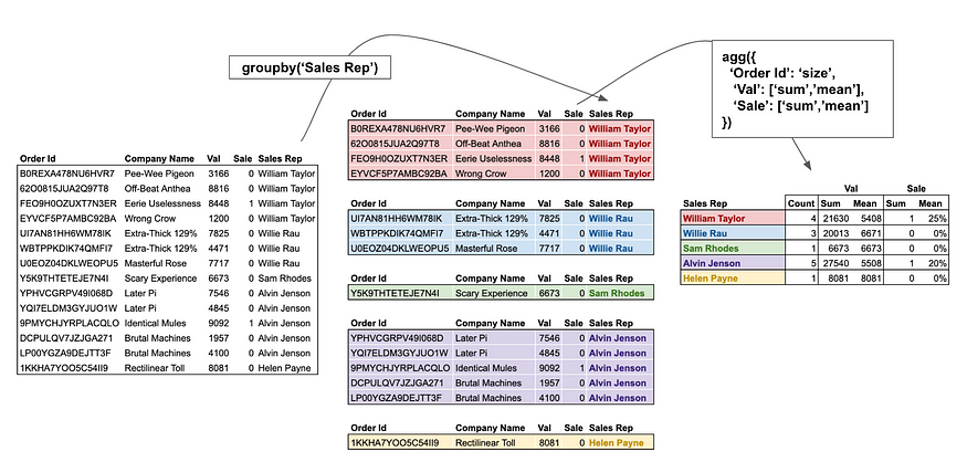
Aggregate is by and large the most powerful of the bunch. Let’s dissect the above image and primarily focus on the righthand part of the process. The following code snippet creates a larger version of the above image.
df.groupby('Sales Rep').agg({
    'Order Id':'size',
    'Val':['sum','mean'],
    'Sale':['sum','mean']
})
We pass a dictionary to the aggregation function, where the keys (i.e. Order Id, Val, Sale) are the columns and the values ('size', ['sum','mean'], ['sum','mean']) are the functions to be applied to the respective columns.
Note that the functions can either be a single function or a list of functions (where then all of them will be applied). Also, note that agg can work with function names (i.e., strings) or actual functions (i.e., Python objects). A non-exhaustive list of functions can be found here. The ones I use most frequently are:
'size': Counts the rows'sum': Sums the column up'mean'/'median': Mean/Median of the column'max'/'min': Maximum/Minimum of the column'idxmax'/'idxmin': Index of the maximum/minimum of the column. Getting the index of the minimal or maximal value is helpful for mapping other columns, i.e., what’s the name of the company per sales rep with the biggest dealpd.Series.nunique: Counts unique values. Note that, unlike the previous functions, this is an actual function and not a string.
pd.NamedAgg
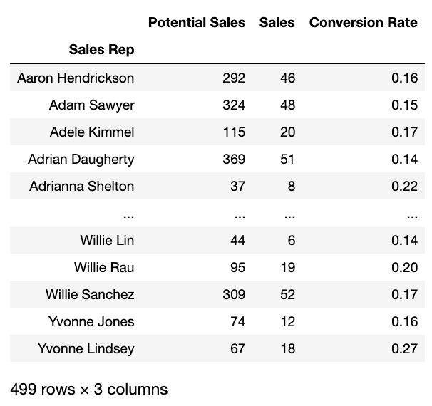
Now, one problem, when applying multiple aggregation functions to multiple columns this way, is that the result gets a bit messy, and there is no control over the column names. In the past, I often found myself aggregating a DataFrame only to rename the results directly afterward. I always found that a bit inefficient. Situations like this are where pd.NamedAgg comes in handy. pd.NamedAgg was introduced in Pandas version 0.25 and allows to specify the name of the target column.
def cr(x):
    return round(np.mean(x),2)

# Long Form: Explictly specifying the NamedAgg
aggregation = {
    'Potential Sales': pd.NamedAgg(column='Val', aggfunc='size'),
    'Sales': pd.NamedAgg(column='Sale', aggfunc='sum'),
    'Conversion Rate': pd.NamedAgg(column='Sale', aggfunc=cr)
}
# Alternative: Since the NamedAgg is just a tuple, we can also pass regular tuples
aggregation = {
    'Potential Sales': ('Val','size'),
    'Sales': ('Sale','sum'),
    'Conversion Rate': ('Sale',cr)
}
df.groupby('Sales Rep').agg(**aggregation)
running the above snippet results in:
C. transform
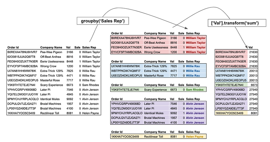
While agg returns a reduced version of the input, transform returns a group-level transformed version of the full data. The new output data has the same length as the input data. For users coming from SQL, think of transform as a window function.
A typical example is to get the percentage of the groups total by dividing by the group-wise sum.
df.groupby('Sales Rep')['Val'].transform(lambda x: x/sum(x))

# OUT:
0        0.004991
1        0.005693
2        0.003976
3        0.000799
4        0.003300
           ...
99995    0.012088
99996    0.000711
99997    0.013741
99998    0.010695
99999    0.001533
Name: Val, Length: 100000, dtype: float64
Unlike agg, transform is typically used by assigning the results to a new column. In our above example, we could do:
df['%'] = df.groupby('Sales Rep')['Val'].transform(
  lambda x: x/sum(x)
)
D. filter
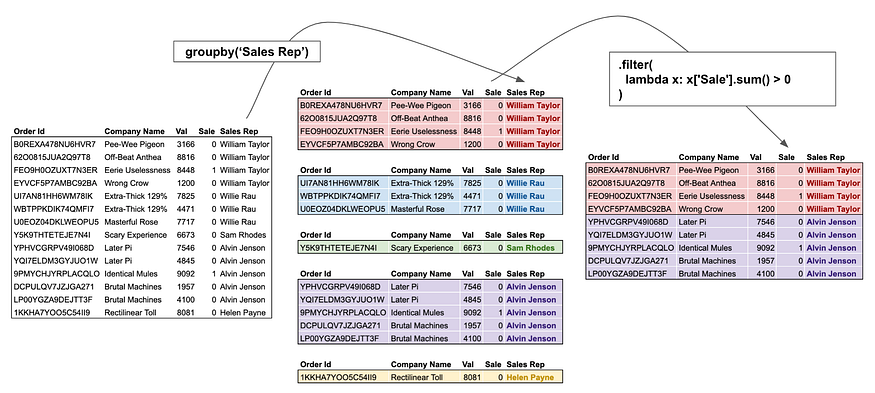
Filter, as the name suggests, does not change the data in any capacity, but instead selects a subset of the data. For users coming from SQL, think of filter as the HAVING condition.
We could for example filter for all sales reps who have at least made 200k:
df.groupby('Sales Rep').filter(
  lambda x: (x['Val'] * x['Sale']).sum() > 200000
)

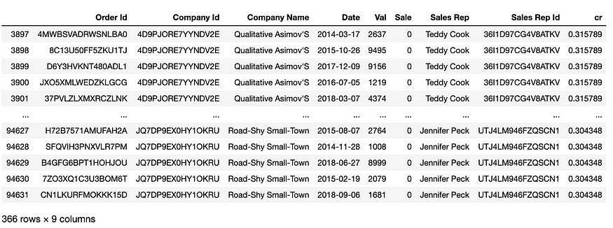
Or all sales Reps with a conversion rate of > 30%:
# Let's add this for verification
df['cr'] = df.groupby('Sales Rep')['Sale'].transform('mean')
df.groupby('Sales Rep').filter(lambda x: x['Sale'].mean() > .3)
Conclusion
In this post, you learned how to group DataFrames like a real Pandas pro. You learned a plethora of ways to group your data. Pandas .groupby() method allows you to analyze, aggregate, filter, and transform your data in many useful ways. Below, you’ll find a quick recap of the Pandas .groupby() method:
- The Pandas
.groupby()method allows you to aggregate, transform, and filter DataFrames - The method works by using split, transform, and apply operations
- You can group data by multiple columns by passing in a list of columns
- You can easily apply multiple aggregations by applying the
.agg()method - You can use the method to transform your data in useful ways, such as calculating z-scores or ranking your data across different groups
The official documentation for the Pandas .groupby() method can be found here.
Resources:
https://pbpython.com/groupby-agg.html
https://towardsdatascience.com/pandas-groupby-aggregate-transform-filter-c95ba3444bbb
https://towardsdatascience.com/pandas-groupby-aggregate-transform-filter-c95ba3444bbb

