Walk-forward optimization for algorithmic trading strategies on cloud architecture

2021-12-26

A guide on PySpark Window Functions with Partition By

2022-02-17

Machine Learning Interview: Sampling and dataset generation

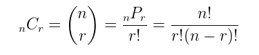
Permutation Formula

A permutation is the choice of r things from a set of n things without replacement and where the order matters.

ⁿP_r = (n!) / (n-r)!

Combination Formula

A combination is the choice of r things from a set of n things without replacement and where order does not matter.

2) What is the difference between sampling with vs. without replacement? Name an example of when you would use one rather than the other.

Sampling with replacement and sampling without replacement are two methods of selecting items from a population.

Sampling with replacement means that after an item is selected, it is put back into the population, so it could be chosen again. In contrast, sampling without replacement means that once an item is selected, it is not put back into the population and cannot be selected again.

An example of sampling with replacement would be selecting a card from a deck, writing down the card, and then returning it to the deck before selecting another card. An example of sampling without a replacement would be selecting a jury for a trial from a pool of potential jurors, where once a person is selected for the jury, they are no longer in the pool of potential jurors.

Which method to use depends on the situation and what you want to accomplish. Sampling with replacement is generally used when the population is very large, and the sample size is relatively small, or when the effect of sampling is minimal. For example, if you are trying to estimate the proportion of a particular type of tree in a large forest, and you are taking only a small sample, then it would make sense to sample with replacement. On the other hand, if you are selecting a team of people for a project, and you want to ensure that everyone has an equal chance of being selected, then you would sample without replacement.

3) Explain Markov chain Monte Carlo sampling.

Markov Chain Monte Carlo (MCMC) is a class of algorithms used to generate samples from a probability distribution that is difficult or impossible to sample directly. The basic idea behind MCMC is to construct a Markov chain whose stationary distribution is the desired probability distribution.

The algorithm works by starting with an initial state and then iteratively proposing new states based on a proposal distribution. The proposed state is accepted with a probability determined by the ratio of the target distribution and the proposal distribution. If the proposed state is accepted, it becomes the new state of the Markov chain, and the process continues. If the proposed state is rejected, the current state remains as the next sample.

Over time, the Markov chain explores the space of possible states and converges to the stationary distribution of the target distribution. The samples generated by the Markov chain can then be used to estimate various properties of the target distribution, such as the mean or variance.

One common application of MCMC sampling is in Bayesian inference. In this context, the target distribution is the posterior distribution of the model parameters given the observed data. MCMC is used to generate samples from the posterior distribution, which can then be used to estimate the posterior mean or to construct credible intervals.

In Markov chain Monte Carlo (MCMC) methods, a proposal distribution is a probability distribution used to generate candidate values for the next step in the Markov chain. The proposal distribution is an important component of the Metropolis-Hastings algorithm, which is a popular MCMC method.

The proposal distribution defines a way to generate a candidate value for the next step in the chain, given the current state of the chain. The candidate value is then accepted or rejected based on the acceptance probability, which is calculated based on the ratio of the posterior distribution of the candidate value and the current state of the chain.

The choice of proposal distribution can have a significant impact on the efficiency of the MCMC algorithm. A good proposal distribution should generate candidate values that are likely to be accepted, while still exploring the space of possible values in an efficient way. Commonly used proposal distributions include normal, uniform, and gamma distributions, among others. The choice of proposal distribution depends on the problem being solved and the characteristics of the posterior distribution being estimated.

Example:

Here’s an example of Markov chain Monte Carlo (MCMC) sampling using the Metropolis-Hastings algorithm:

Suppose we want to estimate the mean of a normal distribution with an unknown mean and variance. We have some prior belief about the distribution of the mean and variance, but we want to update our belief based on some observed data. We can use MCMC sampling to simulate the posterior distribution of the mean and variance.

Let’s say our prior belief about the mean is also normally distributed with mean 0 and variance 1, and our prior belief about the variance is a gamma distribution with shape parameter 2 and rate parameter 1. We observe some data, which is a sample of 10 numbers drawn from a normal distribution with unknown mean and variance.

We can set up our Metropolis-Hastings algorithm to sample from the posterior distribution of the mean and variance, given our prior beliefs and the observed data. We start with some initial guesses for the mean and variance, and then we propose a new value for the mean and variance by adding a small random number to the current value. We calculate the likelihood of the observed data given the proposed mean and variance, and we use Bayes’ rule to calculate the posterior probability of the proposed mean and variance given the observed data and our prior beliefs.

If the posterior probability of the proposed mean and variance is higher than the current value, we accept the proposal as the new value. If the posterior probability is lower, we accept the proposal with a probability proportional to the ratio of the posterior probabilities of the proposed and current values.

We repeat this process for many iterations, and we get a sequence of samples from the posterior distribution. We discard the first few samples to allow the chain to reach equilibrium, and we use the remaining samples to estimate the mean and variance of the posterior distribution. We can also use the samples to compute other quantities of interest, such as the probability that the mean is greater than a certain value or the correlation between the mean and variance.

Here are some common methods used in Markov Chain Monte Carlo (MCMC):

Metropolis-Hastings Algorithm: This is a popular method used to generate a random sample from a target distribution. It is a generalization of the Metropolis algorithm that allows for acceptance of the new state based on a probability distribution.
Gibbs Sampling: This method is used for sampling from a multivariate distribution. In this method, each parameter is sampled conditionally on the values of the other parameters.
Hamiltonian Monte Carlo: This is a more sophisticated MCMC method that is designed to handle distributions that are high-dimensional and/or have complex geometries. It uses Hamiltonian dynamics to generate proposal states that are more likely to be accepted.
Slice Sampling: This method is used for unimodal distributions, where the target distribution is sliced along one dimension, and a sample is drawn from the intersection of the slice and the target distribution.
Reversible Jump MCMC: This method is used when the dimensionality of the target distribution is unknown. It allows for the transition between different dimensions of the target distribution.
Sequential Monte Carlo: This is a method that involves generating a sequence of weighted samples that approximate the target distribution. It is useful when the target distribution is complex or has a large number of dimensions.
Importance Sampling: This method involves drawing samples from an easy-to-sample proposal distribution and then reweighting them to approximate the target distribution. It is useful when the target distribution is difficult to sample directly.

There are many other methods used in MCMC, but these are some of the most common.

The Challenge of Probabilistic Inference

Calculating a quantity from a probabilistic model is referred to more generally as probabilistic inference, or simply inference.

For example, we may be interested in calculating an expected probability, estimating the density, or other properties of the probability distribution. This is the goal of the probabilistic model, and the name of the inference performed often takes on the name of the probabilistic model, e.g. Bayesian Inference is performed with a Bayesian probabilistic model.

The direct calculation of the desired quantity from a model of interest is intractable for all but the most trivial probabilistic models. Instead, the expected probability or density must be approximated by other means.

For most probabilistic models of practical interest, exact inference is intractable, and so we have to resort to some form of approximation.

— Page 523, Pattern Recognition and Machine Learning, 2006.

The desired calculation is typically a sum of a discrete distribution of many random variables or integral of a continuous distribution of many variables and is intractable to calculate. This problem exists in both schools of probability, although is perhaps more prevalent or common with Bayesian probability and integrating over a posterior distribution for a model.

Bayesians, and sometimes also frequentists, need to integrate over possibly high-dimensional probability distributions to make inference about model parameters or to make predictions. Bayesians need to integrate over the posterior distribution of model parameters given the data, and frequentists may need to integrate over the distribution of observables given parameter values.

— Page 1, Markov Chain Monte Carlo in Practice, 1996.

The typical solution is to draw independent samples from the probability distribution, then repeat this process many times to approximate the desired quantity. This is referred to as Monte Carlo sampling or Monte Carlo integration, named for the city in Monaco that has many casinos.

The problem with Monte Carlo sampling is that it does not work well in high-dimensions. This is firstly because of the curse of dimensionality, where the volume of the sample space increases exponentially with the number of parameters (dimensions).

Secondly, and perhaps most critically, this is because Monte Carlo sampling assumes that each random sample drawn from the target distribution is independent and can be independently drawn. This is typically not the case or intractable for inference with Bayesian structured or graphical probabilistic models.

What Is Markov Chain Monte Carlo

The solution to sampling probability distributions in high-dimensions is to use Markov Chain Monte Carlo, or MCMC for short.

The most popular method for sampling from high-dimensional distributions is Markov chain Monte Carlo or MCMC

— Page 837, Machine Learning: A Probabilistic Perspective, 2012.

Like Monte Carlo methods, Markov Chain Monte Carlo was first developed around the same time as the development of the first computers and was used in calculations for particle physics required as part of the Manhattan project for developing the atomic bomb.

Monte Carlo

Monte Carlo is a technique for randomly sampling a probability distribution and approximating a desired quantity.

Monte Carlo algorithms, [….] are used in many branches of science to estimate quantities that are difficult to calculate exactly.

— Page 530, Artificial Intelligence: A Modern Approach, 3rd edition, 2009.

Monte Carlo methods typically assume that we can efficiently draw samples from the target distribution. From the samples that are drawn, we can then estimate the sum or integral quantity as the mean or variance of the drawn samples.

A useful way to think about a Monte Carlo sampling process is to consider a complex two-dimensional shape, such as a spiral. We cannot easily define a function to describe the spiral, but we may be able to draw samples from the domain and determine if they are part of the spiral or not. Together, a large number of samples drawn from the domain will allow us to summarize the shape (probability density) of the spiral.

Markov Chain

Markov chain is a systematic method for generating a sequence of random variables where the current value is probabilistically dependent on the value of the prior variable. Specifically, selecting the next variable is only dependent upon the last variable in the chain.

A Markov chain is a special type of stochastic process, which deals with characterization of sequences of random variables. Special interest is paid to the dynamic and the limiting behaviors of the sequence.

— Page 113, Markov Chain Monte Carlo: Stochastic Simulation for Bayesian Inference, 2006.

Consider a board game that involves rolling dice, such as snakes and ladders (or chutes and ladders). The roll of a die has a uniform probability distribution across 6 stages (integers 1 to 6). You have a position on the board, but your next position on the board is only based on the current position and the random roll of the dice. Your specific positions on the board form a Markov chain.

Another example of a Markov chain is a random walk in one dimension, where the possible moves are 1, -1, chosen with equal probability, and the next point on the number line in the walk is only dependent upon the current position and the randomly chosen move.

At a high level, a Markov chain is defined in terms of a graph of states over which the sampling algorithm takes a random walk.

— Page 507, Probabilistic Graphical Models: Principles and Techniques, 2009.

Markov Chain Monte Carlo

Combining these two methods, Markov Chain and Monte Carlo, allows random sampling of high-dimensional probability distributions that honors the probabilistic dependence between samples by constructing a Markov Chain that comprise the Monte Carlo sample.

MCMC is essentially Monte Carlo integration using Markov chains. […] Monte Carlo integration draws samples from the the required distribution, and then forms sample averages to approximate expectations. Markov chain Monte Carlo draws these samples by running a cleverly constructed Markov chain for a long time.

— Page 1, Markov Chain Monte Carlo in Practice, 1996.

Specifically, MCMC is for performing inference (e.g. estimating a quantity or a density) for probability distributions where independent samples from the distribution cannot be drawn, or cannot be drawn easily.

As such, Monte Carlo sampling cannot be used.

Instead, samples are drawn from the probability distribution by constructing a Markov Chain, where the next sample that is drawn from the probability distribution is dependent upon the last sample that was drawn. The idea is that the chain will settle on (find equilibrium) on the desired quantity we are inferring.

Yet, we are still sampling from the target probability distribution with the goal of approximating a desired quantity, so it is appropriate to refer to the resulting collection of samples as a Monte Carlo sample, e.g. extent of samples drawn often forms one long Markov chain.

The idea of imposing a dependency between samples may seem odd at first, but may make more sense if we consider domains like the random walk or snakes and ladders games, where such dependency between samples is required.

Markov Chain Monte Carlo Algorithms

There are many Markov Chain Monte Carlo algorithms that mostly define different ways of constructing the Markov Chain when performing each Monte Carlo sample.

The random walk provides a good metaphor for the construction of the Markov chain of samples, yet it is very inefficient. Consider the case where we may want to calculate the expected probability; it is more efficient to zoom in on that quantity or density, rather than wander around the domain. Markov Chain Monte Carlo algorithms are attempts at carefully harnessing properties of the problem in order to construct the chain efficiently.

This sequence is constructed so that, although the first sample may be generated from the prior, successive samples are generated from distributions that provably get closer and closer to the desired posterior.

— Page 505, Probabilistic Graphical Models: Principles and Techniques, 2009.

MCMC algorithms are sensitive to their starting point, and often require a warm-up phase or burn-in phase to move in towards a fruitful part of the search space, after which prior samples can be discarded and useful samples can be collected.

Additionally, it can be challenging to know whether a chain has converged and collected a sufficient number of steps. Often a very large number of samples are required and a run is stopped given a fixed number of steps.

… it is necessary to discard some of the initial samples until the Markov chain has burned in, or entered its stationary distribution.

— Page 838, Machine Learning: A Probabilistic Perspective, 2012.

The most common general Markov Chain Monte Carlo algorithm is called Gibbs Sampling; a more general version of this sampler is called the Metropolis-Hastings algorithm.

Let’s take a closer look at both methods.

Gibbs Sampling Algorithm

The Gibbs Sampling algorithm is an approach to constructing a Markov chain where the probability of the next sample is calculated as the conditional probability given the prior sample.

Samples are constructed by changing one random variable at a time, meaning that subsequent samples are very close in the search space, e.g. local. As such, there is some risk of the chain getting stuck.

The idea behind Gibbs sampling is that we sample each variable in turn, conditioned on the values of all the other variables in the distribution.assumptions

— Page 838, Machine Learning: A Probabilistic Perspective, 2012.

Gibbs Sampling is appropriate for those probabilistic models where this conditional probability can be calculated, e.g. the distribution is discrete rather than continuous.

… Gibbs sampling is applicable only in certain circumstances; in particular, we must be able to sample from the distribution P(Xi | x-i). Although this sampling step is easy for discrete graphical models, in continuous models, the conditional distribution may not be one that has a parametric form that allows sampling, so that Gibbs is not applicable.

— Page 515, Probabilistic Graphical Models: Principles and Techniques, 2009.

Metropolis-Hastings Algorithm

The Metropolis-Hastings Algorithm is appropriate for those probabilistic models where we cannot directly sample the so-called next state probability distribution, such as the conditional probability distribution used by Gibbs Sampling.

Unlike the Gibbs chain, the algorithm does not assume that we can generate next-state samples from a particular target distribution.

— Page 517, Probabilistic Graphical Models: Principles and Techniques, 2009.

Instead, the Metropolis-Hastings algorithm involves using a surrogate or proposal probability distribution that is sampled (sometimes called the kernel), then an acceptance criterion that decides whether the new sample is accepted into the chain or discarded.

They are based on a Markov chain whose dependence on the predecessor is split into two parts: a proposal and an acceptance of the proposal. The proposals suggest an arbitrary next step in the trajectory of the chain and the acceptance makes sure the appropriate limiting direction is maintained by rejecting unwanted moves of the chain.

— Page 6, Markov Chain Monte Carlo: Stochastic Simulation for Bayesian Inference, 2006.

The acceptance criterion is probabilistic based on how likely the proposal distribution differs from the true next-state probability distribution.

The Metropolis-Hastings Algorithm is a more general and flexible Markov Chain Monte Carlo algorithm, subsuming many other methods.

For example, if the next-step conditional probability distribution is used as the proposal distribution, then the Metropolis-Hastings is generally equivalent to the Gibbs Sampling Algorithm. If a symmetric proposal distribution is used like a Gaussian, the algorithm is equivalent to another MCMC method called the Metropolis algorithm.

https://machinelearningmastery.com/markov-chain-monte-carlo-for-probability/

4) If you need to sample from high-dimensional data, which sampling method would you choose?

If I need to sample from high-dimensional data, I would choose the Markov Chain Monte Carlo (MCMC) method. MCMC is a popular and effective approach for sampling from complex, high-dimensional distributions. It works by constructing a Markov chain that has the target distribution as its equilibrium distribution, and then using the chain to generate a sequence of samples that approximate the target distribution. The key advantage of MCMC is that it can be used to sample from distributions that are difficult to sample from directly, such as those with many variables or complicated dependencies.

5) Suppose we have a classification task with many classes. An example is when you have to predict the next word in a sentence — the next word can be one of many, many possible words. If we have to calculate the probabilities for all classes, it’ll be prohibitively expensive. Instead, we can calculate the probabilities for a small set of candidate classes. This method is called candidate sampling. Name and explain some of the candidate sampling algorithms. Hint: check out this great article on candidate sampling by the TensorFlow team.

Sampled softmax is a candidate sampling algorithm used to approximate the softmax function in large classification problems. In the softmax function, the probability of each class is calculated by dividing the exponential of the score of that class by the sum of exponentials of scores for all classes. However, this calculation can become prohibitively expensive in high-dimensional classification problems with a large number of classes.

Sampled softmax approximates the probability distribution by randomly sampling a small number of classes instead of considering all possible classes. The algorithm works by dividing the score of a particular class by the sum of scores of a small randomly selected set of classes plus one. The size of the randomly selected set of classes is a hyperparameter of the algorithm.

Sampled softmax can be more efficient than calculating the softmax function directly, especially in large classification tasks with a very large number of classes. However, it introduces additional noise into the calculation of probabilities, which can affect the quality of the model.

Here is a numerical example of how sampled softmax works:

Suppose we have a language model that is trained to predict the next word in a sentence given the previous words. The vocabulary size of the language model is 10,000 words.

Instead of calculating the probabilities of all 10,000 words at each step, we can randomly sample a small number of words (say, 100) from the vocabulary to calculate the softmax probabilities. Let’s assume we want to predict the next word given the context “The cat is”. Here are the counts of the 10 most frequent words in the vocabulary that follow this context:

cat: 500
sitting: 200
running: 150
sleeping: 100
eating: 50
… (rest of the vocabulary)

To use sampled softmax, we randomly sample 100 words from the vocabulary, including the target word if it is in the 100 words. Let’s say that the sampled words are: cat, sitting, running, sleeping, eating, and 95 other words.

We then calculate the softmax probabilities only for these 100 words, rather than all 10,000 words. The probabilities for the sampled words are calculated using the softmax function as follows:

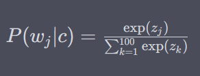
where $z_j$ is the logit (unnormalized log-probability) of word $w_j$, given the context $c$.

We can then use the sampled softmax probabilities to compute the loss and update the model’s parameters using backpropagation. This approach reduces the computational cost of the softmax calculation, making it feasible to train the model on large vocabularies.

Noise Contrastive Estimation (NCE) is a candidate sampling algorithm used to estimate the parameters of a probability distribution. The idea behind NCE is to transform the problem of estimating the parameters of a probability distribution into a binary classification problem. Specifically, given a data point and a set of candidate samples, NCE trains a binary classifier to distinguish the true data point from the candidate samples. The algorithm then uses the parameters of the classifier to estimate the parameters of the probability distribution.

Here’s a simplified example of how NCE works:

Suppose we have a dataset of words and we want to estimate the probability distribution of the next word given a context. Let’s say we have a context consisting of the words “the”, “quick”, and “brown”, and we want to estimate the probability distribution of the next word from a vocabulary of 10,000 words. Instead of computing the probabilities for all 10,000 words, we can use NCE to select a small set of candidate words and estimate the probabilities for those words.

To use NCE, we first choose a noise distribution Q over the vocabulary. The noise distribution should be chosen to be similar to the true data distribution, but can be simpler to compute. For example, we can choose Q to be a uniform distribution over all 10,000 words.

Next, for each context word, we sample a set of K noise words from the noise distribution Q. In our example, let’s say we choose K = 5 and sample the words “dog”, “cat”, “jumped”, “over”, and “lazy” as noise words for the context word “brown”.

We then define a binary classification problem, where the goal is to distinguish the true data point (the word that actually follows the context) from the K noise words. We use logistic regression to train the classifier, with the input being a feature vector representing the context and the candidate word, and the output being a binary label indicating whether the word is a noise word or the true data point.

Finally, we use the parameters of the logistic regression classifier to estimate the probabilities of the candidate words. Specifically, the probability of a candidate word given the context is proportional to the probability that the classifier assigns to that word being the true data point, after normalizing over all candidate words.

Overall, NCE allows us to estimate the parameters of a probability distribution in a more computationally efficient way, by selecting a small set of candidate samples and training a binary classifier to distinguish the true data point from the noise samples.

7) Suppose you want to build a model to classify whether a Reddit comment violates the website’s rule. You have 10 million unlabeled comments from 10K users over the last 24 months and you want to label 100K of them.

How would you sample 100K comments to label?
Suppose you get back 100K labeled comments from 20 annotators and you want to look at some labels to estimate the quality of the labels. How many labels would you look at? How would you sample them?

Hint: This article on different sampling methods and their use cases might help.

There are different strategies for sampling 100K comments from 10 million unlabeled comments. One common approach is to use stratified sampling, where you divide the unlabeled comments into different strata based on some criteria, such as the user who posted the comment or the subreddit where the comment was posted. Then, you randomly sample a certain number of comments from each stratum. This approach ensures that you have a representative sample of comments from different subpopulations.

To estimate the quality of the labels provided by the annotators, you can use a technique called annotation agreement analysis. This involves comparing the annotations from multiple annotators and measuring the level of agreement among them. By sampling a subset of the labeled comments and examining the labels, you can assess the quality of the annotations.

Here’s an approach you can follow to determine the number of labels to look at and how to sample them:

Calculate the inter-annotator agreement: Compute the agreement metric, such as Cohen’s kappa or Fleiss’ kappa, to measure the level of agreement among the annotators. This step will give you an overall sense of the agreement quality.
Determine the desired confidence level: Decide on the level of confidence you want to achieve in estimating the quality of the labels. This could be based on the desired level of precision or the acceptable level of error.
Calculate the required sample size: Use statistical methods to determine the number of labels you need to sample in order to achieve the desired confidence level. The sample size calculation takes into account the level of agreement, the desired confidence level, and the population size.
Randomly sample the labels: Once you have determined the required sample size, randomly select that number of labeled comments from the 100,000 labeled dataset. Random sampling ensures that the selected labels are representative of the overall dataset and reduces bias.
Evaluate the sampled labels: Examine the labels of the sampled comments to assess the quality of the annotations. You can calculate the agreement among the sampled annotators and compare it to the overall agreement calculated earlier. This comparison will give you an estimate of the quality of the labels.
Repeat if necessary: If the initial sample does not provide enough confidence or if the quality of the labels is not satisfactory, you can repeat the process by sampling additional comments until you achieve the desired confidence level.

The specific number of labels to look at will depend on the level of confidence you require and the results of the sample size calculation. It’s important to strike a balance between obtaining sufficient information about the annotation quality and minimizing the effort required for manual inspection.

By following this approach, you can estimate the quality of the labels provided by the annotators by examining a representative subset of the labeled comments.

The number of labels to look at for estimating the quality of the labels depends on several factors, such as the desired level of precision and confidence, the variability of the annotators’ labels, and the budget and time constraints. A common approach is to use a statistical sampling method, such as random sampling or stratified sampling, to select a representative subset of the labeled data to review.

The sample size can be determined using sample size calculation methods, which take into account the variability of the data, the desired level of precision and confidence, and the population size. For example, if the goal is to estimate the annotators’ agreement on a binary classification task with a 95% confidence level and a margin of error of 5%, a sample size of around 385 labeled comments would be needed, assuming a population size of 100K labeled comments and a 50-50 split of positive and negative comments.

Once the sample is selected, the quality of the labels can be assessed using different metrics, such as inter-annotator agreement, accuracy, or F1 score, depending on the task and the evaluation criteria. The results of the quality assessment can then be used to adjust the labels or the annotation process or to inform the model training and evaluation.

The number of labels to look at and the sampling strategy would depend on the specific goals of the analysis and the level of confidence desired in the quality estimates. Here are a few general guidelines:

Determine the required level of confidence: To determine how many labels to look at, you need to decide on the level of confidence you want to have in your quality estimates. If you need a high level of confidence, you may need to look at more labels than if you need a lower level of confidence.
Choose a representative sample: Once you have determined the number of labels to look at, you need to choose a representative sample of labels. One way to do this is to randomly sample the labels from the entire set of 100K labeled comments.
Stratified sampling: Another option is to use stratified sampling, where you sample from specific subsets of the data based on relevant factors, such as the annotator, the label, or the sentiment of the comment. This can help ensure that the sample is representative of the overall dataset and can be useful when you suspect that some subsets of the data may have lower quality labels than others.
Decide on which labels to look at: Once you have a representative sample, you need to decide which labels to look at. You may want to focus on labels that have low inter-annotator agreement or labels that are particularly important for your analysis.
Check for quality: Finally, to estimate the quality of the labels, you will need to check the labels for accuracy and consistency across annotators. You can use metrics such as inter-annotator agreement or confusion matrices to assess the quality of the labels.

8) Suppose you work for a news site that historically has translated only 1% of all its articles. Your coworker argues that we should translate more articles into Chinese because translations help with the readership. On average, your translated articles have twice as many views as your non-translated articles. What might be wrong with this argument?

Hint: think about selection bias.

One potential issue with the argument that translating more articles into Chinese will help with readership is the possibility of selection bias. Specifically, the translated articles that have been published so far may not be a representative sample of the entire set of articles that could be translated.

For example, the translated articles may have been selected based on their perceived appeal to a Chinese-speaking audience, which could introduce a bias towards articles that are more likely to be popular or relevant to that audience. Similarly, the translated articles may have been selected based on the availability of translators or other resources, rather than their potential appeal to a Chinese-speaking audience.

If the translated articles that have been published so far are not a representative sample of the entire set of articles that could be translated, then the observed higher viewership of translated articles may not be indicative of the potential impact of translating more articles. To address this, it may be necessary to conduct a systematic analysis of the entire set of articles and identify those that are most likely to be of interest to a Chinese-speaking audience, and then translate those articles.

Moreover, it is also possible that the higher viewership of translated articles is not solely due to their being translated, but also due to other factors such as their topic, relevance, or quality. To account for these factors, it may be necessary to compare the viewership of translated and non-translated articles that are similar in terms of these factors.

Selection bias is a type of bias that occurs when the sample or population being studied is not representative of the larger population, either due to how the sample was chosen or because of characteristics of the sample itself. This can lead to inaccurate or misleading conclusions because the sample does not reflect the true characteristics of the population.

Examples of selection bias include:

Volunteer bias: When individuals who choose to participate in a study are not representative of the general population. For example, a study on a new drug may only recruit volunteers who are particularly interested in the drug or who are in better health, leading to inaccurate conclusions about the drug’s effectiveness in the general population.
Non-response bias: When individuals who do not respond to a survey or study are systematically different from those who do respond. For example, if a survey on voting intentions only receives responses from people who are strongly committed to a particular party, the results may not be representative of the wider population.
Sampling bias: When the method used to select a sample is flawed or not random. For example, if a pollster only interviews people at a certain location, such as a shopping mall, the sample may not be representative of the wider population.
Survivorship bias: When only survivors or those who have completed a particular task are studied, leading to a biased view of the success rate or difficulty of the task. For example, a study on the success rates of new businesses that only looks at successful businesses may not provide an accurate picture of the challenges faced by new businesses.
Healthy user bias: When studies are conducted on people who are in better health, leading to a biased view of the effectiveness of treatments or interventions. For example, a study on the effectiveness of a new exercise program that only recruits individuals who are already physically fit may not provide an accurate view of the program’s effectiveness for individuals with a range of fitness levels.

9) How to determine whether two sets of samples (e.g. train and test splits) come from the same distribution?

https://towardsdatascience.com/how-dis-similar-are-my-train-and-test-data-56af3923de9b

To determine whether two sets of samples come from the same distribution, you can perform a statistical test for comparing distributions. There are several methods to compare distributions, including parametric and nonparametric tests.

Parametric tests assume that the data come from a specific distribution, such as a normal distribution, and compare the parameters of the distribution between the two samples. Common parametric tests include the t-test, ANOVA, and the Kolmogorov-Smirnov test.

Nonparametric tests do not assume a specific distribution and instead compare the ranks or order of the data between the two samples. Common nonparametric tests include the Wilcoxon rank-sum test, the Mann-Whitney U test, and the Kruskal-Wallis test.

Here are the general steps to compare two sets of samples:

Choose a statistical test that is appropriate for your data and research question.
Determine the null hypothesis, which states that the two samples come from the same distribution.
Calculate the test statistic, which measures the difference between the two samples.
Calculate the p-value, which indicates the probability of obtaining the observed test statistic under the null hypothesis.
Compare the p-value to the significance level, typically set at 0.05, to determine whether to reject or fail to reject the null hypothesis.

If the p-value is less than the significance level, you can reject the null hypothesis and conclude that the two samples come from different distributions. If the p-value is greater than the significance level, you fail to reject the null hypothesis and conclude that the two samples come from the same distribution.

To determine whether two sets of samples, such as train and test splits, come from the same distribution, there are several statistical tests that can be used. Here are a few common methods:

Kolmogorov-Smirnov test: This test compares the empirical cumulative distribution functions (CDFs) of the two sets of samples. If the CDFs are significantly different, then the two sets of samples may come from different distributions.
Anderson-Darling test: This test is similar to the Kolmogorov-Smirnov test, but it places more weight on differences in the tails of the distribution. It is more sensitive to differences in the tails than the Kolmogorov-Smirnov test.
Chi-squared test: This test compares the observed frequencies of each value or bin in the two sets of samples to the expected frequencies if the two sets of samples came from the same distribution. If the observed and expected frequencies are significantly different, then the two sets of samples may come from different distributions.
Visual inspection: This method involves plotting histograms or density plots of the two sets of samples and visually inspecting them to see if they look similar. If the histograms or density plots look different, then the two sets of samples may come from different distributions.
Domain knowledge: Sometimes, domain knowledge can be used to determine whether the samples come from the same distribution. For example, if the train data contains only images of dogs and the test data contains only images of cats, it is clear that the two samples come from different distributions.
Cross-validation: Another approach is to use cross-validation to assess the performance of the model on multiple train-test splits. If the performance of the model is consistent across multiple splits, it suggests that the train and test data are likely to come from the same distribution.

10) How do you know you’ve collected enough samples to train your ML model?

https://towardsdatascience.com/how-do-you-know-you-have-enough-training-data-ad9b1fd679ee

https://machinelearningmastery.com/much-training-data-required-machine-learning/

11) How to determine outliers in your data samples? What to do with them?

Outliers are observations in a dataset that are significantly different from other observations. There are various ways to determine outliers in data samples, including:

Visual inspection: A simple way to identify outliers is to plot the data and look for any observations that are far away from the other data points.
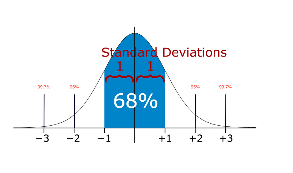
Statistical methods: Statistical methods such as the z-score and interquartile range (IQR) can be used to detect outliers. Observations that fall outside a certain threshold, such as three standard deviations from the mean or outside the IQR, can be considered outliers.
Machine learning algorithms: Some machine learning algorithms, such as DBSCAN clustering, Isolation Forests, and decision trees, can also be used to detect outliers.
Robust Random Cut Forest:
Random Cut Forest (RCF) algorithm is Amazon’s unsupervised algorithm for detecting anomalies.

Once outliers have been identified, there are several options for what to do with them:

Remove them: In some cases, outliers may be due to measurement error or other anomalies, and removing them may be appropriate. However, it is important to be careful when removing data as it can affect the overall distribution and accuracy of the analysis.
Keep them: In some cases, outliers may be legitimate data points and removing them may result in the loss of important information. In this case, keeping them and addressing their impact on the analysis may be more appropriate.
Transform the data: If outliers are skewing the distribution of the data, transforming the data may help to reduce their impact. This can include using a logarithmic or square root transformation or normalizing the data.

Dealing with Outliers

Deleting the values: You can delete the outliers if you know that the outliers are wrong or if the reason the outlier was created is never going to happen in the future. For example, there is a data set of peoples ages and the usual ages lie between 0 to 90 but there is data entry off the age 150 which is nearly impossible. So, we can safely drop the value that is 150.
Changing the values: We can also change the values in the cases when we know the reason for the outliers. Consider the previous example for measurement or instrument errors where we had 10 voltmeters out of which one voltmeter was faulty. Here what we can do is that we can take another set of readings using a correct voltmeter and replace them with the readings that were taken by the faulty voltmeter.
Data transformation: Data transformation is useful when we are dealing with highly skewed data sets. By transforming the variables, we can eliminate the outliers for example taking the natural log of a value reduces the variation caused by the extreme values. This can also be done for data sets that do not have negative values.
Using different analysis methods: You could also use different statistical tests that are not as much impacted by the presence of outliers – for example, using median to compare data sets as opposed to mean or use of equivalent nonparametric tests etc.
Valuing the outliers: In case there is a valid reason for the outlier to exist and it is a part of our natural process, we should investigate the cause of the outlier as it can provide valuable clues that can help you better understand your process performance. Outliers may be hiding precious information that could be invaluable to improve your process performance. You need to take the time to understand the special causes that contributed to these outliers. Fixing these special causes can give you significant boost in your process performance and improve customer satisfaction. For example, normal delivery of orders takes 1-2 days, but a few orders took more than a month to complete. Understanding the reason why it took a month and fixing this process can help future customers as they would not be impacted by such large wait times.

https://regenerativetoday.com/a-complete-guide-for-detecting-and-dealing-with-outliers/

12) When should you remove duplicate training samples? When shouldn’t you? What happens if we accidentally duplicate every data point in your train set or in your test set?

Duplicate training samples should be removed when they do not provide any additional information to the model and only increase the computational load during training. Duplicate samples can arise due to various reasons, such as data collection processes or preprocessing steps.

However, there are some cases where duplicate samples may be useful for the model, such as when dealing with imbalanced datasets or when specific samples need to be emphasized. In these cases, removing duplicate samples may lead to a loss of information.

Ultimately, the decision to remove duplicate samples should be made on a case-by-case basis, taking into account the goals of the model, the nature of the data, and the available computational resources.

If every data point in the train or test set is accidentally duplicated, it can lead to biased results and overfitting. The model will learn to predict the duplicated samples perfectly, but it may not generalize well to unseen data.

Furthermore, duplicated samples will increase the computational load during training and evaluation, potentially leading to longer training times and higher resource requirements.

To avoid this issue, it is essential to carefully inspect the data and ensure that there are no accidental duplications before training and testing the model.

13) In your dataset, two out of 20 variables have more than 30% missing values. What would you do? How might techniques that handle missing data make selection bias worse? How do you handle this bias?

If two out of 20 variables in the dataset have more than 30% missing values, several options can be considered:

Imputation: Use imputation techniques to fill in the missing values. There are various imputation techniques available, such as mean imputation, median imputation, regression imputation, and K-nearest neighbor imputation. The choice of imputation technique will depend on the nature of the data and the goals of the analysis.
Deletion: Delete the missing values or the variables with high missing rates. However, this can lead to a loss of information, especially if the variables with missing values are critical to the analysis.
Feature engineering: Create new features from the existing data to replace the variables with missing values. This approach may require domain expertise and may not be feasible in all cases.
Use of models that can handle missing data: Use models that can handle missing data, such as tree-based models or Bayesian methods.

The choice of approach will depend on the nature of the data, the goals of the analysis, and the available computational resources.

How might techniques that handle missing data make selection bias worse? How do you handle this bias?

Techniques that handle missing data can make selection bias worse if the missing data are not missing at random (MAR). For example, if the missing values are related to certain characteristics of the data, such as age, gender, or income, and these characteristics are also related to the outcome variable, the imputation or deletion of the missing data can introduce bias.

To handle this bias, it is essential to understand the reasons for the missing data and the potential relationships between the missing data and the outcome variable. If the missing data are not MAR, then imputation or deletion techniques may not be appropriate. Instead, more sophisticated techniques, such as multiple imputation or inverse probability weighting, can be used to account for the bias.

Multiple imputation involves creating multiple imputed datasets, each of which includes plausible values for the missing data. The analysis is then performed on each of the imputed datasets, and the results are combined to produce an overall estimate. This approach can reduce the bias introduced by the missing data.

Inverse probability weighting involves weighting the observations based on the probability of the observation being missing, conditional on the observed data. This approach can adjust for the non-randomness of the missing data and reduce bias.

Overall, handling missing data and selection bias requires a careful analysis of the data and consideration of the appropriate techniques to use. It is important to understand the potential sources of bias and to use appropriate methods to account for them.

Missing Completely at Random (MCAR): Missing data is said to be MCAR if the probability of missingness is the same for all cases, both those with missing values and those without. In other words, the missingness is unrelated to any observed or unobserved variables in the data. MCAR is considered the least problematic type of missing data because it does not introduce any bias into the analysis.
Missing at Random (MAR): Missing data is said to be MAR if the probability of missingness depends on observed data but not on the missing data itself. In other words, the probability of missingness is related to the observed variables in the data. MAR is a common type of missing data, and it can introduce bias into the analysis if it is not handled properly.
Missing Not at Random (MNAR): Missing data is said to be MNAR if the probability of missingness depends on the missing data itself. In other words, the missingness is related to unobserved variables in the data, and the missing values may be systematically different from the observed values. MNAR is the most problematic type of missing data because it can introduce bias into the analysis, and it is difficult to handle properly.

Examples:

Missing Completely at Random (MCAR): Suppose you are conducting a survey of a population, and the survey data includes a question about income. However, some respondents did not answer the question about income because they accidentally skipped it or didn’t feel comfortable answering. If the probability of missingness is the same for all respondents, regardless of their income or any other characteristic, then the missing data is MCAR.
Missing at Random (MAR): Suppose you are analyzing medical data to investigate the relationship between smoking and lung cancer. In the data, smoking status is missing for some patients. However, it is observed that patients who are older are more likely to have missing smoking status. In this case, the probability of missingness is related to an observed variable (age) but not the missing variable (smoking status). The missing data is therefore MAR.
Missing Not at Random (MNAR): Suppose you are conducting a study on employee productivity, and you ask employees to self-report their productivity levels. However, some employees refuse to report their productivity levels because they believe it will impact their job security. In this case, the missingness is related to an unobserved variable (job security) and the missing values may be systematically different from the observed values. The missing data is therefore MNAR.

14) Why is randomization important when designing experiments (experimental design)?

Randomization is an important component of experimental design because it helps to ensure that the differences observed between groups are due to the treatment being studied and not to other factors that may influence the outcome.

When designing an experiment, researchers usually divide the participants into two or more groups, with each group receiving a different treatment or intervention. Randomization involves randomly assigning participants to these groups, which helps to ensure that the groups are comparable at the start of the experiment. By randomly assigning participants to the treatment and control groups, any differences between the groups are likely to be due to chance, rather than to other factors such as age, gender, or socioeconomic status. This reduces the risk of bias and ensures that the results are more generalizable to the population of interest.

Randomization can also help to reduce the impact of confounding variables. Confounding variables are variables that are related to both the treatment and the outcome, and if they are not controlled for, they can lead to erroneous conclusions about the effectiveness of the treatment. By randomly assigning participants to groups, the distribution of confounding variables is likely to be similar across the groups, which reduces their impact on the outcome.

In summary, randomization is important in experimental design because it helps to ensure that the groups are comparable at the start of the experiment, reduces the risk of bias, and reduces the impact of confounding variables, all of which increase the validity and reliability of the results.

15) How would class imbalance affect your model? Why is it hard for ML models to perform well on data with class imbalance?

Class imbalance can affect a model’s performance by biasing it towards the majority class. This is because the model is trained on an unbalanced dataset where one class is significantly more represented than the other, resulting in the model being less sensitive to the minority class. As a result, the model might perform well on the majority class, but poorly on the minority class, leading to a high false-negative rate or low recall.
ML models struggle with class imbalance because they are trained to minimize overall error or maximize accuracy. In an imbalanced dataset, the majority class will dominate the accuracy metric, and the model will be optimized for that class. As a result, the model may learn to predict the majority class accurately, but fail to capture the minority class’s nuances and patterns.

https://towardsdatascience.com/how-to-deal-with-imbalanced-classification-without-re-balancing-the-data-8a3c02353fe3

16) Imagine you want to build a model to detect skin legions from images. In your training dataset, only 1% of your images show signs of legions. After training, your model seems to make a lot more false negatives than false positives. What are some of the techniques you’d use to improve your model?

When facing a scenario where your model shows a high number of false negatives (missed skin lesions) compared to false positives (incorrectly identifying non-lesion areas as lesions), you can employ several techniques to improve its performance. Here are some techniques you can consider:

Collect more diverse and representative data: Since only 1% of your training images show signs of lesions, collecting more data, particularly positive examples (images with skin lesions), can help balance the class distribution and provide the model with more information to learn from. This can help reduce the false negative rate.
Data augmentation: Apply data augmentation techniques to increase the variability of your training data. Techniques such as rotation, scaling, flipping, and adding noise can create additional training examples, making the model more robust to different variations in skin lesion images.
Adjust the decision threshold: By default, models often use a probability threshold of 0.5 for classification. However, you can adjust this threshold to control the trade-off between false negatives and false positives. Decreasing the threshold can increase the sensitivity (recall) of the model, reducing false negatives but potentially increasing false positives.
Resampling techniques: Utilize resampling techniques, such as oversampling the minority class (lesion images) or undersampling the majority class (non-lesion images), to create a more balanced training dataset. This can help the model focus on the minority class and improve its ability to detect lesions.
Model optimization and tuning: Experiment with different models and architectures that might better capture the characteristics of skin lesions. You can try more advanced models or modify existing ones by adjusting hyperparameters, such as learning rate, regularization techniques, or using pre-trained models for transfer learning.
Ensemble learning: Employ ensemble techniques, such as bagging or boosting, to combine multiple models’ predictions. Ensemble methods can often improve overall performance and reduce both false positives and false negatives.
Post-processing techniques: Apply post-processing techniques to the model’s output probabilities or predictions. For example, you can use morphological operations like dilation or erosion to refine the predicted lesion regions, or consider using post-processing algorithms like Conditional Random Fields (CRFs) to incorporate spatial information and improve segmentation accuracy.
Error analysis: Analyze the false negative cases in detail to identify patterns or specific challenges in detecting lesions. This analysis can help you gain insights into the limitations of the current model and guide further improvements, such as targeted data collection or feature engineering.

It’s important to iterate and experiment with different combinations of these techniques, as their effectiveness can vary depending on the specific problem and dataset. Regular evaluation and validation of the model’s performance on a separate test dataset can help gauge the impact of these techniques and guide further refinements.

17) Training data leakage: Imagine you’re working with a binary task where the positive class accounts for only 1% of your data. You decide to oversample the rare class then split your data into train and test splits. Your model performs well on the test split but poorly in production. What might have happened?

In this scenario, oversampling the rare class can cause the model to overfit on the minority class, leading to poor performance in production. This is because oversampling can introduce bias and noise into the training data, causing the model to learn patterns that do not generalize well to new data. Therefore, the model may have become overly specialized to the training set and not able to generalize to new data in production.

Additionally, oversampling can increase the risk of overfitting since it creates multiple copies of the same data points, increasing the likelihood that the model will learn the idiosyncrasies of those data points. This can lead to poor generalization and low performance in production.

To mitigate these issues, it’s essential to use cross-validation and evaluation metrics that can detect overfitting and ensure that the model is generalizing well to new data.

18) You want to build a model to classify whether a comment is spam or not spam. You have a dataset of a million comments over the period of 7 days. You decide to randomly split all your data into the train and test splits. Your co-worker points out that this can lead to data leakage. How?

If your model performs well on the test split but poorly in production, it suggests that there might be training data leakage, where information from the test set or other unseen data has inadvertently leaked into the training process. This can lead to overly optimistic performance during testing, as the model has unintentionally learned to exploit patterns specific to the test data. Here are a few potential reasons for this discrepancy:

Oversampling before splitting: If you oversampled the rare positive class before splitting your data into train and test sets, it is possible that some of the duplicated positive examples ended up in both the training and test sets. This leakage can cause the model to have artificially inflated performance on the test set since it has already seen similar examples during training.
Information leakage through feature engineering: If you performed feature engineering or preprocessing steps based on the entire dataset (including the test set) before splitting, information from the test set could have influenced the training process. For instance, if you calculated statistics or derived features using the entire dataset, the model might have indirectly learned specific properties of the test data.
Target leakage through feature selection: If you used feature selection techniques based on the target variable (such as univariate feature selection or feature importance), and these techniques were applied to the entire dataset before splitting, it could introduce target leakage. The model might have indirectly learned relationships between certain features and the target variable that are specific to the test data, leading to inflated performance on the test set.
Time-based or temporal leakage: If your dataset has a temporal component, it’s possible that there is temporal leakage. For example, if the rare positive class occurs more frequently during certain time periods or has a specific temporal pattern, the model might inadvertently learn these patterns during training. However, these patterns might not generalize well to new, unseen data in production.

To address these issues and mitigate training data leakage, it is crucial to follow best practices:

Split the data before oversampling: Ensure that you split the data into train and test sets before applying any oversampling techniques. This helps to maintain the integrity of the separation between training and evaluation data.
Perform feature engineering and preprocessing after the split: Conduct feature engineering and preprocessing steps based only on the training data. This ensures that the model is learning patterns from the training set alone and does not inadvertently utilize information from the test set.
Use cross-validation: Employ cross-validation techniques, such as k-fold cross-validation, to evaluate your model’s performance more robustly. Cross-validation helps to assess the generalization capability of the model across multiple folds and provides a more reliable estimate of its performance.

By carefully handling the data splitting, feature engineering, and evaluation processes, you can minimize the risk of training data leakage and improve the model’s performance in real-world production scenarios.

https://stats.stackexchange.com/questions/488856/does-using-a-random-train-test-split-lead-to-data-leakage

19) How does data sparsity affect your models?

Data sparsity refers to the situation where some features in a dataset have very few or no observations. In other words, some features have zero values for most of the data points. Data sparsity can have a significant impact on the performance of machine learning models. Here are a few ways it can affect models:

Overfitting: When a model has too few examples for a particular feature, it may learn to overemphasize the importance of that feature, even if it is not relevant. This can lead to overfitting, where the model is too specialized to the training data and does not generalize well to new data.
Bias: If the data is too sparse, some features may have too few observations to be significant in predicting the target variable. As a result, the model may be biased towards certain features and not take into account other important factors.
Reduced Accuracy: Data sparsity can also reduce the overall accuracy of a model. This is because there may not be enough data to fully capture the complexity of the underlying relationships between the features and the target variable.
Slow training time: Sparse data can cause the model training to be very slow. This is because the model needs to work harder to make sense of the data and find relevant patterns.

To overcome data sparsity, techniques such as feature engineering, dimensionality reduction, and data augmentation can be applied. Additionally, algorithms that are designed to handle sparse data such as tree-based models, gradient boosting, and deep learning models can be used.

Methods for Dealing with Sparse Features

1. Removing features from the model

Sparse features can introduce noise, which the model picks up and increase the memory needs of the model. To remedy this, they can be dropped from the model. For example, rare words are removed from text mining models, or features with low variance are removed. However, sparse features that have important signals should not be removed in this process.

LASSO regularization can be used to decrease the number of features. Rule-based methods like setting a variance threshold for including features in the model might also be useful.

2. Make the features dense

Principal component analysis (PCA): PCA methods can be used to project the features into the directions of the principal components and select from the most important components.
Feature hashing: In feature hashing, sparse features can be binned into the desired number of output features using a hash function. Care must be taken to choose a generous number of output features to prevent hash collisions.

3. Using models that are robust to sparse features

Some versions of machine learning models are robust towards sparse data and may be used instead of changing the dimensionality of the data. For example, the entropy-weighted k-means algorithm is better suited to this problem than the regular k-means algorithm.

20) Feature leakage: What are some causes of feature leakage? Why does normalization help prevent feature leakage? How do you detect feature leakage?

Feature leakage occurs when information from the target variable (the variable you’re trying to predict) leaks into the features used to train a machine learning model. Some causes of feature leakage include:

Using data that is not available at the time of prediction. For example, including future information in the training set.
Including data that is a result of the target variable. For example, using the total revenue generated by a customer as a feature to predict whether they will buy a product in the future.
Data preprocessing that is based on the entire dataset, rather than just the training set. For example, scaling the data before splitting it into training and test sets.

Normalization can help prevent feature leakage by ensuring that each feature has a similar scale and range. This is important because some machine learning algorithms (such as distance-based algorithms like k-nearest neighbors) are sensitive to differences in scale between features. If one feature has a much larger scale than another, it can dominate the learning process and cause the algorithm to focus too heavily on that feature. Normalization can help prevent this by scaling all features to a similar range.
Detecting feature leakage can be challenging, but there are a few methods you can use to check if it is occurring in your dataset:

Examine the data for any features that are strongly correlated with the target variable. If a feature is strongly correlated with the target, it may be a sign of leakage.
Check for any features that are generated after the target variable is known. For example, if you’re predicting customer churn and one of the features is the number of days since a customer cancelled their account, that is likely a sign of leakage.
Use cross-validation to check the performance of your model on different subsets of the data. If your model performs significantly worse on new data than on the training set, that may indicate feature leakage.
Normalization can help prevent feature leakage by scaling the features to a consistent range, which can help remove any hidden relationships between features. For example, if two features have a similar range but different units of measurement, they may appear to be strongly correlated even if they are not. By normalizing the features, these hidden relationships can be revealed and accounted for during model training.
Detecting feature leakage can be challenging, but there are several approaches that can be used. One approach is to carefully examine the training set and look for any instances where data from the future or other sources of information that would not be available during inference time are included. Another approach is to look for features that are strongly correlated with the target variable, as this may indicate that the model is overfitting to the training set. Additionally, feature importance measures such as permutation importance or SHAP values can be used to identify features that are highly predictive but may be leaking information from the target variable.

Feature leakage, a.k.a. data leakage or target leakage, causes predictive models to appear more accurate than they really are, ranging from overly optimistic to completely invalid. The cause is highly correlated data – where the training data contains information you are trying to predict.

How to Minimize Feature Leakage:

Remove data that could not be known at the time of prediction.
Perform data cross-validation.
If you suspect a variable is leaky, remove it and run again.
Hold back a validation data set.
Consider near-perfect model accuracy a warning sign.
Check variables of importance for overly predictive features.

https://towardsdatascience.com/data-leakage-in-machine-learning-how-it-can-be-detected-and-minimize-the-risk-8ef4e3a97562

Data leakage or information leakage, occurs when information from the test or evaluation data unintentionally leaks into the training process, leading to overly optimistic performance metrics. Feature leakage can significantly impact the accuracy and reliability of machine learning models, as it violates the fundamental principle of evaluating models on unseen data. Here are a few common scenarios that can cause feature leakage:

Using Future Information: Training a model using features or data that would not be available in a real-world scenario can lead to feature leakage. For example, using future timestamps or variables that are determined after the target variable (e.g., using a customer’s purchase history to predict their current behavior) can introduce information that the model would not have access to in a real application.
Target Leakage: Target leakage occurs when features that are directly influenced by the target variable or contain information about the target are included in the training data. This can artificially inflate the model’s performance during training but fail to generalize to new data. For instance, including a feature that indicates whether a customer eventually made a purchase when predicting whether they will make a purchase can lead to target leakage.
Data Preprocessing Leakage: Applying preprocessing steps, such as scaling or feature transformations, based on the entire dataset (including the test set) before splitting into train and test can introduce leakage. This is because the model gains information from the test set during the preprocessing stage, leading to an overly optimistic evaluation.
Train-Test Data Leakage: When feature engineering or preprocessing steps are performed using information from both the training and test sets, it can lead to leakage. For instance, calculating statistics (mean, standard deviation, etc.) using the entire dataset, or using the entire dataset to impute missing values, can introduce information from the test set into the training process.
Information Leakage through Feature Selection: Conducting feature selection techniques (such as univariate feature selection or feature importance) based on the entire dataset before splitting can cause feature leakage. The model may inadvertently learn relationships between features and the target variable that are specific to the test set, leading to inflated performance during evaluation.

To avoid feature leakage and ensure a fair evaluation of your model’s performance, it is important to follow best practices:

Split Data Properly: Split your dataset into separate and distinct training, validation, and test sets. Ensure that no information from the validation or test sets is used during the model development process, including feature engineering, preprocessing, and hyperparameter tuning.
Preserve Temporal Order: If your data has a temporal component, ensure that the temporal order is maintained during the data splitting process. The model should not have access to future information during training.
Perform Feature Engineering and Preprocessing after Data Split: Conduct feature engineering, data preprocessing, and scaling based only on the training data. The same transformations should be applied consistently to the validation and test sets.
Use Cross-Validation: Instead of relying solely on a single train-test split, employ cross-validation techniques such as k-fold cross-validation. This helps to assess the model’s performance on multiple validation sets and provides a more robust estimate of its generalization ability.

By being mindful of potential feature leakage and following proper data splitting and modeling practices, you can ensure that your machine learning models are evaluated accurately and provide reliable performance estimates on unseen data.

21) Suppose you want to build a model to classify whether a tweet spreads misinformation. You have 100K labeled tweets over the last 24 months. You decide to randomly shuffle on your data and pick 80% to be the train split, 10% to be the valid split, and 10% to be the test split. What might be the problem with this way of partitioning?

One potential problem with randomly shuffling the data and splitting it into the train, validation, and test sets is that it may not preserve the temporal order of the data. In the case of the tweet classification problem, the temporal order of the tweets could be important, as misinformation trends and patterns may change over time.

By randomly shuffling the data and splitting it into train, validation, and test sets, there is a risk that the model will be trained on tweets from one period of time and tested on tweets from another period of time, which could lead to poor generalization performance. For example, the model may perform well on tweets from the training period but poorly on tweets from the testing period due to changes in the patterns of misinformation.

To address this issue, it may be better to split the data based on time rather than randomly. For example, we could split the data into training and validation sets based on tweets from the first 22 months and use the remaining 2 months of tweets for the test set. This way, the model is trained on tweets from an earlier time period and tested on tweets from a more recent time period, which is more likely to reflect the real-world scenario.

22) You’re building a neural network and you want to use both numerical and textual features. How would you process those different features?

https://towardsdatascience.com/how-to-combine-textual-and-numerical-features-for-machine-learning-in-python-dc1526ca94d9

https://realpython.com/python-keras-text-classification/

When processing both numerical and textual features in a neural network, it is necessary to transform the features into a format that the network can understand and use for making predictions. The processing of numerical and textual features is usually different, and the following steps can be taken to handle them separately:

For numerical features:

Scaling: Numerical features should be scaled to have similar ranges, typically by using techniques such as mean normalization or standardization. This step is important because features with larger ranges might dominate other features during the learning process.
Encoding: In some cases, numerical features can be directly used in the neural network without any encoding. However, if the numerical values represent categories or classes, they should be encoded as one-hot vectors, where each category is represented by a binary vector.

For textual features:

Tokenization: Textual features need to be broken down into smaller units called tokens. This step is typically done by splitting the text into words or subwords, depending on the language and the specific task.
Embedding: After tokenization, each token is represented by a dense vector of fixed size, which is called an embedding. The embedding is typically learned from the data using techniques such as word2vec or GloVe.
Padding: Textual features can have different lengths, so they need to be padded or truncated to a fixed length to be fed into the neural network.

After processing the numerical and textual features separately, the features can be combined by concatenating them into a single input vector that can be fed into the neural network. Alternatively, multiple neural network branches can be used to process the different types of features separately and then merge them at some point in the network architecture. The specific processing steps and architecture would depend on the specific problem and the nature of the data.

23) Your model has been performing fairly well using just a subset of features available in your data. Your boss decided that you should use all the features available instead. What might happen to the training error? What might happen to the test error?

If we use all the available features instead of just a subset, we might observe the following effects:

Training Error: The training error may decrease or stay the same as we increase the number of features. This is because more features allow the model to capture more complex patterns in the data. However, it is also possible that the training error may increase as the model starts to overfit to the noise in the data due to the increased complexity.
Test Error: The test error may initially decrease as we add more features because the model has access to more information about the data. However, at some point, adding more features can lead to the curse of dimensionality, where the model starts to overfit to the training data and performs poorly on new, unseen data. This is because the more dimensions we have to describe our data, the sparser the space becomes, and the further apart the data points are from each other. As a result, the model may start to fit to noise in the training data, leading to poor generalization performance on the test data.

Because of this inherent sparsity, we end up overfitting, when we add more features to our data, which means we need more data to avoid sparsity — and that’s the curse of dimensionality: as the number of features increases, our data become sparser, which results in overfitting, and we therefore need more data to avoid it.

In general, it is recommended to use feature selection or feature engineering techniques to identify the most important features for the task at hand and avoid using too many irrelevant or redundant features. This can help prevent overfitting and improve the model’s generalization performance.

The curse of dimensionality refers to the phenomenon where the difficulty of certain computational problems increases exponentially with the number of dimensions (or features) in the data. In other words, as the number of dimensions increases, the volume of the feature space increases so rapidly that the available data becomes increasingly sparse, and the distance between data points becomes larger, making it more difficult to find meaningful patterns or relationships in the data.

This can cause several issues in machine learning, such as overfitting, difficulty in feature selection, and slow convergence of optimization algorithms. Additionally, it can make it more difficult to generalize well to new, unseen data, as the model may become too complex and overfit to the training data.

To mitigate the curse of dimensionality, it is important to carefully consider which features to use in the model, use techniques such as dimensionality reduction (e.g., PCA, t-SNE), regularization, or feature selection, and use larger amounts of data if possible to provide a denser sampling of the feature space.

The curse of dimensionality can have a significant effect on overfitting in machine learning. When dealing with high-dimensional data, the risk of overfitting increases, meaning that the model may become too complex and fit the training data too closely, leading to poor generalization performance on new, unseen data.

One of the main reasons why high-dimensional data can increase the risk of overfitting is that it can lead to a model with a large number of parameters relative to the number of available training examples. This can result in a model that is too complex and can memorize the training data instead of learning the underlying patterns.

To address overfitting in high-dimensional data, techniques such as regularization or feature selection can be used to reduce the complexity of the model and prevent it from overfitting. Regularization methods, such as L1 or L2 regularization, penalize large weights in the model, which can help to reduce the number of parameters and simplify the model. Feature selection methods, such as backward or forward feature selection, can be used to identify the most relevant features and remove irrelevant or noisy features from the model, which can also help to reduce its complexity and improve generalization performance. Additionally, using larger amounts of data and carefully monitoring the training and test errors can help to prevent overfitting in high-dimensional data.

An increase in the number of dimensions of a dataset means there are more entries in the vector of features that represents each observation in the corresponding Euclidean space. We measure the distance in a vector space using Euclidean distance.

The Euclidean distance between 2-dimensional vectors with Cartesian coordinates p = (p1, p2, …, pn) and q = (q1, q2, …, qn) is computed using the familiar formula:

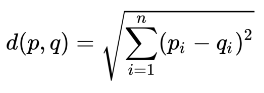
Hence, each new dimension adds a non-negative term to the sum, so the distance increases with the number of dimensions for distinct vectors. In other words, as the number of features grows for a given number of observations, the feature space becomes increasingly sparse; that is, less dense or emptier. On the flip side, the lower data density requires more observations to keep the average distance between data points the same.

Similar to the above figures, below shows how many data points we need to maintain the average distance of 10 observations uniformly distributed on a line. It increases exponentially from 10¹ in a single dimension to 10² in two and 10³ in three dimensions, as the data needs to expand by a factor of 10 each time we add a new dimension:

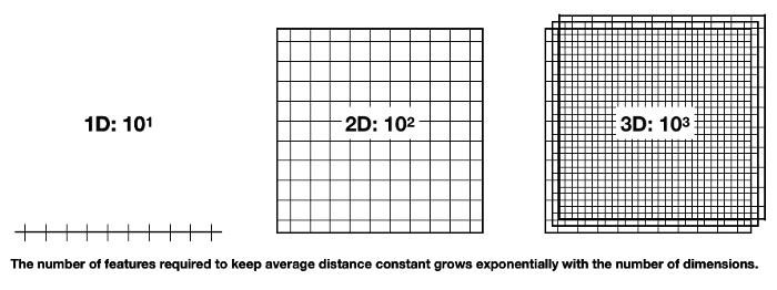
From the above figure, it is proven that with the increase in dimensions, mean distance increases rapidly. Hence the higher the dimensions, the more data is needed to overcome the curse of dimensionality!

Read more about the curse of dimensionality:

https://towardsdatascience.com/the-curse-of-dimensionality-5673118fe6d2

https://builtin.com/data-science/curse-dimensionality