A simple tutorial on Sampling Importance and Monte Carlo with Python codes

Introduction

In this post, I’m going to explain the importance sampling. Importance sampling is an approximation method instead of a sampling method. It shows up in machine learning topics as a trick. It is derived from a little mathematic transformation and is able to formulate the problem in another way.

The content of this post is mainly based on this fantastic YouTube tutorial. You can find the Jupyter notebook for this post here.

What is Monte Carlo?

It’s difficult to understand importance sampling in a vacuum. It will make a lot more sense if we motivate it from the perspective of Monte Carlo methods. Let’s dive right into these techniques are concerned with one extremely important test that shows up a ton in machine learning: Calculating Expectations. Without going into too much detail, expectations are very frequently the answers that many of our ML algorithms are seeking. They show up when fitting models, doing probability queries, summarizing model performance, and training a reinforcement learning agent. 

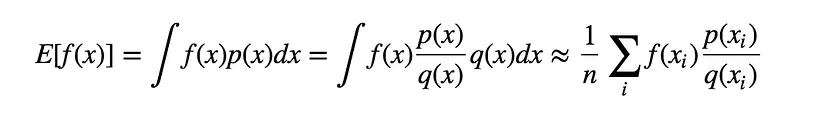
Now mathematically that means we are interested in calculating this:

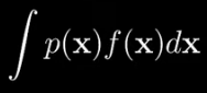
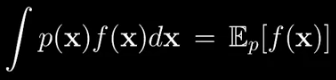
where x is a continuous random vector. Boldface means it is a vector and p(x) is the probability density of x. f(x) is just some scalar function of x we happen to be interested in.  Now you should think of this as the probability-weighted average of f(x) over the entire space where x lives to communicate that. It is often written like this:

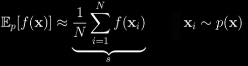
As an aside if x were discrete then this integral would turn into a sum. None of the concepts really change for the discrete case. We’ll continue with the continuous case. Now the problem is sometimes, in fact, a lot of the time, this integral is impossible to calculate exactly. It is because the dimension of x is high so the space that lives within is exponentially huge and we have no hope of adding everything up within it. This is where Monte Carlo methods come in. The idea is to merely approximate the expectation with an average. 

This average says we need to collect N samples of x from the distribution p, plug those into f, and take their average. It turns out that as N gets large this thing approaches our answer. For the sake of brevity, let’s call this sum s. 

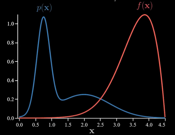
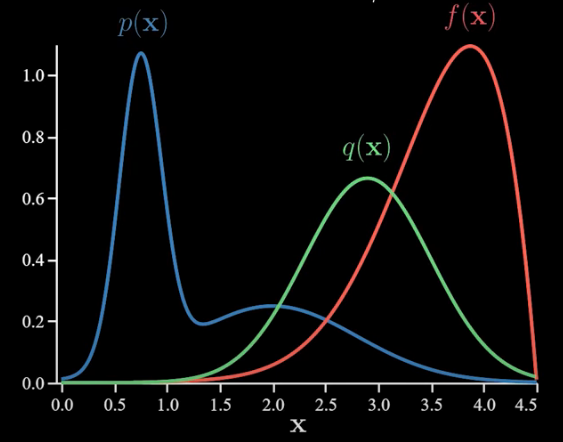
Let’s play with a one-dimensional example. Let’s say p(x) and f(x) are as below:

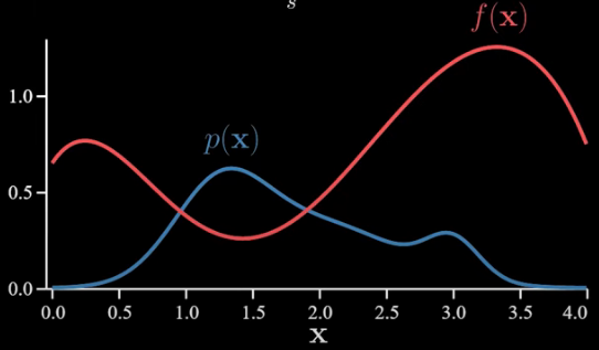
In this case, things are simple enough that we can calculate the answer exactly. To do that, we look at the product function and calculate the area under the purple curve. 

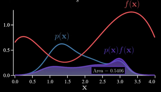
This is the exact value (0.5406). Please use your imagination and pretend we cannot actually calculate the area this way because in the general case, it can be impossible. So instead, let’s approximate this area using the Monte Carlo method. First, we sample x‘s from p(x) and then plug those into f(x) the average of these is an approximation to the integral.

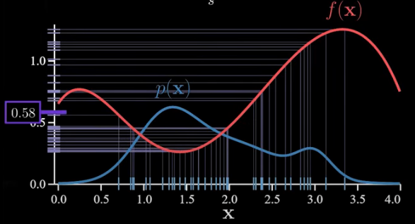
To emphasize, the core of Monte Carlo is to say the average of lines mapped on the y-axis (0.58) is an approximation to the area under the purple curve in the previous image (0.54). I’m not proving that but trust me it’s true and very important frankly. It’s more important than importance sampling!

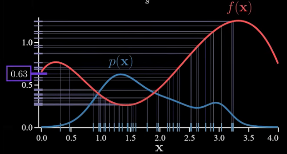
One thing to point out is that the value of average s is random. If we were to resample everything we’d get a new value for s each time. For example, with a different set of values for samples, we have another value for s as follows:

This means that our sample average has its own distribution. Let’s check that out. Let’s say the true expectation we’d like to estimate is as below:

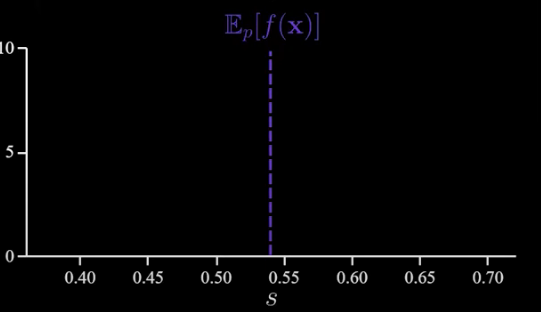
Let’s say we repeat our estimate many times giving us many s‘s. Now we’re in a better position to view the distribution of s.

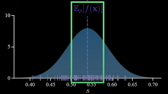
Now to avoid confusion this distribution is just useful for a theoretical understanding of applications. We only get one sample of s. Keep that in mind as I will talk about this thing. The first thing to notice here is the distribution is centered on the true expectation. This is a critical property. When we have this property we say that “our estimate is unbiased”.

Also looking at this distribution, we can see that the variance of s something which tells you about the width of this distribution matters a lot.

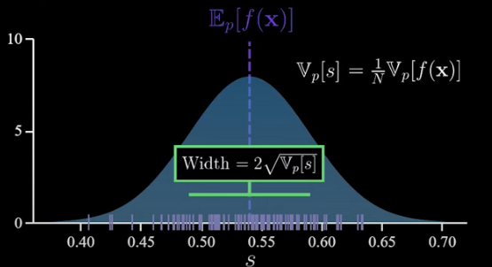
It gives us a sense of how off a single estimate is likely to be from the truth. Now it turns out the variance of s is the variance of f(x) scaled down by N.

One other thing to notice. This distribution is a normal distribution. Where did that come from? Well, that’s the Central Limit Theorem. It’s a magical and super famous result and in this case, it says it doesn’t matter what p(x) or f(x) is, as N gets large this will get closer and closer to a normal distribution. In fact, we can summarize this by writing:

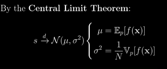
The Central Limit Theorem says:

The distribution of s approaches the normal as N gets large. The mean of that normal is the expectation we are trying to calculate and its variance is the variance of f(x) scaled down by N.

What is the importance sampling?

We start by introducing a new distribution q(x). As we’ll see this is something we get to choose and again we are interested in the same expectation as before. We had earlier noted this still involves p(x). Now here’s a trick. The trick is to multiply the term within the integral by q(x)/q(x) which is just equal to 1.

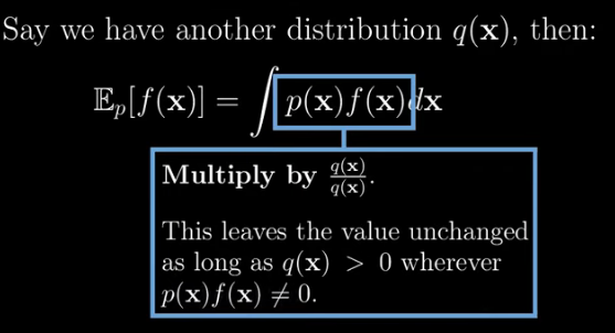
We can do this without damaging anything as long as q(x) is greater than 0 whenever p(x) *f(x) is non-zero.

That gives us the following new integral.

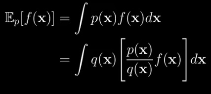
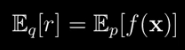
Looking at how I’ve bracketed things we can see that it’s the probability-weighted average of a new function where the probability is given by q(x) instead of p(x). So just like we did earlier, we can write that like this:

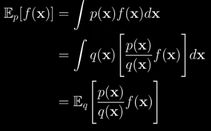
This says:

The p(x) probability weighted average of f(x) is equal to the q(x) probability weighted average of f(x) times the ratio of p(x)/q(x) densities.

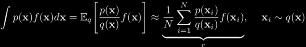
Now if we look at this and we recall the Monte Carlo, we can estimate this with samples from q(x).

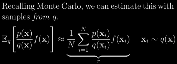
What I mean by that is the original expectation we’re interested in is approximately equal to this new average:

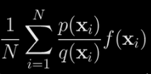
where the x_i‘s are sampled from q(x). Let’s call this new average r.

What’s the advantage of using this?

First, it’s unbiased just like in the previous case:

Second, it has a new possibly improved variance. That is the variance of r which gives us a sense of how off from the truth a single sample of r is likely to be is the variance of f(x) times the density ratio where samples are generated according to q(x) scaled down by N. The hope is we can choose q(x) such that this variance is less than the variance we dealt with earlier. Now, to do that, it turns out q(x) should say x‘s are likely wherever the absolute value of p(x)*f(x) is high.

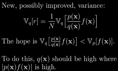
That’s a key result that I’m not proving but it kind of makes sense when you recognize that we are trying to estimate the area under the p(x) times f(x) curve got it.

It’s about time we do an example to help. Here is a little summary of the core ideas we’re demonstrating.

Let’s do an example where importance sampling will reduce the variance quite a bit in particular. Let’s say p(x) and f(x) are as follows:

As a point of reference, let’s calculate several estimates using Monte Carlo without importance sampling:

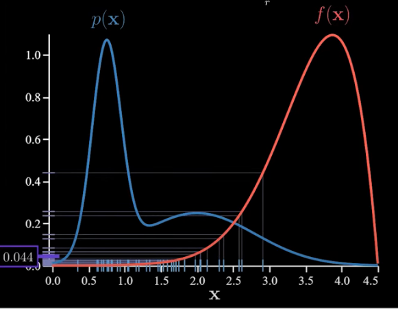
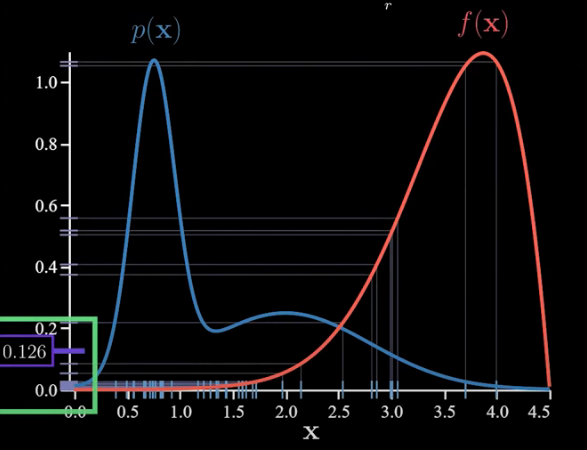
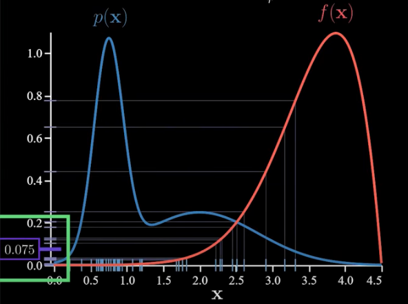
Notice how much our estimate is bouncing around. That is high variance. This is because f(x) is large only in rare events under p(x). So a small set of samples have an outsized impact on the average.

Now importance sampling can help us here because we can make it sample the more important regions more frequently. In particular, I’ll make q(x) like the below:

But now if we’d like to use q samples we need to adjust the f(x) function. So let’s do that by multiplying it by the density ratio which gives us this:

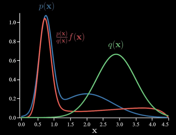
To declutter things a bit I’ll drop p(x).

now after this adjustment, we can proceed just like we did with the plain Monte Carlo. That is we sample from q(x) pass those into the density ratio adjusted f(x) and then calculate their average. This is our new estimate (0.083):

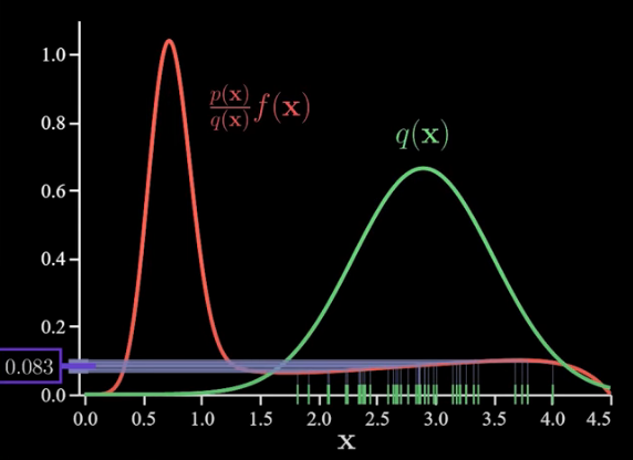
The whole point is if we repeat this process we’ll get something that bounces around less (less variance) than if we sampled the previous way. That’s the whole idea the variance is reduced and with a single estimate, we expect to be less wrong.

How to choose the new distribution q(x) in Importance Sampling?

How are we supposed to choose q(x) in practice if its best answer depends on p(x) and f(x) which are supposedly difficult to work with?

That is indeed tricky and the answers aren’t very satisfying. The hope is that we’ll know a few things about p(x) and f(x) which will guide us. Maybe we know where f(x) is high or maybe we can pick a q(x) that merely approximates p(x). it’s very much an art. Also fair warning, it’s very easy to do a terrible job at selecting q(x), especially in high dimensions. The symptom of that will be the density ratio will vary wildly over the samples and the majority of them will be very small. This means your average will be effectively determined by a small number of samples making it high variance not good.

Importance Sampling with Python code

Let’s recap what we’ve learned so far.

Consider a scenario you are trying to calculate an expectation of function f(x), where x ~ p(x), is subjected to some distribution. We have the following estimation of expectation:

The Monte Carlo sampling method is to simply sample x from the distribution p(x) and take the average of all samples to get an estimation of the expectation. If p(x) is very hard to sample from, we can estimate the expectation based on some known and easily sampled distribution q(x). It comes from a simple transformation of the formula:

where x is sampled from distribution q(x) and q(x) should not be 0. In this way, estimating the expectation is able to sample from another distribution q(x), and p(x)/q(x) is called sampling ratio or sampling weight, which acts as a correction weight to offset the probability sampling from a different distribution.

Another thing we need to talk about is the variance of estimation:

where in this case, X is f(x)p(x)/q(x) , so if p(x)/q(x) is large, this will result in a large variance, which we definitely hope to avoid. On the other hand, it is also possible to select proper q(x) that results in an even smaller variance. Let’s get into a Python example.

Python Example

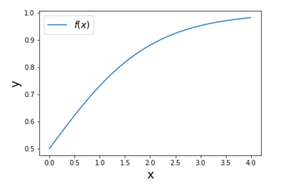
First, let’s define function f(x) and sample distribution:

def f_x(x):
    return 1/(1 + np.exp(-x))

The curve of f(x) looks like this:

Now let’s define the distribution of p(x) and q(x) :

def distribution(mu=0, sigma=1):
    # return probability given a value
    distribution = stats.norm(mu, sigma)
    return distribution
    
# pre-setting
n = 1000

mu_target = 3.5
sigma_target = 1
mu_appro = 3
sigma_appro = 1

p_x = distribution(mu_target, sigma_target)
q_x = distribution(mu_appro, sigma_appro)

For simplicity reasons, here both p(x) and q(x) are normal distributions, you can try to define some p(x)  that is very hard to sample from. In our first demonstration, let’s set two distributions close to each other with similar means (3 and 3.5) and the same sigma 1:

Now we are able to compute the true value sampled from distribution p(x):

s = 0
for i in range(n):
    # draw a sample
    x_i = np.random.normal(mu_target, sigma_target)
    s += f_x(x_i)
print("simulate value", s/n)

where we get an estimation of 0.954. Now let’s sample from q(x) and see how it performs:

value_list = []
for i in range(n):
    # sample from different distribution
    x_i = np.random.normal(mu_appro, sigma_appro)
    value = f_x(x_i)*(p_x.pdf(x_i) / q_x.pdf(x_i))
    
    value_list.append(value)

Notice that here x_i  is sampled from the approximate distribution q(x), and we get an estimation of 0.949 and a variance of 0.304. See that we are able to get the estimate by sampling from a different distribution!

Comparison

The distribution q(x) might be too similar to p(x) that you probably doubt the ability of importance sampling, now let’s try another distribution:

# pre-setting
n = 5000

mu_target = 3.5
sigma_target = 1
mu_appro = 1
sigma_appro = 1

p_x = distribution(mu_target, sigma_target)
q_x = distribution(mu_appro, sigma_appro)

with histogram:

Here we set n to 5000, when the distribution is dissimilar, in general, we need more samples to approximate the value. This time we get an estimation value of 0.995, but a variance of 83.36.

The reason comes from p(x)/q(x), as two distributions are too different from each other could result in a huge difference in this value, thus increasing the variance. The rule of thumb is to define q(x) where p(x)|f(x)|  is large.

Here is the full code:

import numpy as np
import scipy.stats as stats
import matplotlib.pyplot as plt
import seaborn as sns


def f_x(x):
    return 1/(1 + np.exp(-x))


def distribution(mu=0, sigma=1):
    # return probability given a value
    distribution = stats.norm(mu, sigma)
    return distribution


if __name__ == "__main__":
    # pre-setting
    n = 1000

    mu_target = 3.5
    sigma_target = 1
    mu_appro = 3
    sigma_appro = 1

    p_x = distribution(mu_target, sigma_target)
    q_x = distribution(mu_appro, sigma_appro)

    plt.figure(figsize=[10, 4])

    sns.distplot([np.random.normal(mu_target, sigma_target) for _ in range(3000)], label="distribution $p(x)$")
    sns.distplot([np.random.normal(mu_appro, sigma_appro) for _ in range(3000)], label="distribution $q(x)$")

    plt.title("Distributions", size=16)
    plt.legend()

    # value
    s = 0
    for i in range(n):
        # draw a sample
        x_i = np.random.normal(mu_target, sigma_target)
        s += f_x(x_i)
    print("simulate value", s / n)

    # calculate value sampling from a different distribution

    value_list = []
    for i in range(n):
        # sample from different distribution
        x_i = np.random.normal(mu_appro, sigma_appro)
        value = f_x(x_i) * (p_x.pdf(x_i) / q_x.pdf(x_i))

        value_list.append(value)

    print("average {} variance {}".format(np.mean(value_list), np.var(value_list)))

    # pre-setting different q(x)
    n = 5000

    mu_target = 3.5
    sigma_target = 1
    mu_appro = 1
    sigma_appro = 1

    p_x = distribution(mu_target, sigma_target)
    q_x = distribution(mu_appro, sigma_appro)

    plt.figure(figsize=[10, 4])

    sns.distplot([np.random.normal(mu_target, sigma_target) for _ in range(3000)], label="distribution $p(x)$")
    sns.distplot([np.random.normal(mu_appro, sigma_appro) for _ in range(3000)], label="distribution $q(x)$")

    plt.title("Distributions", size=16)
    plt.legend()

    # calculate value sampling from a different distribution

    value_list = []
    # need larger steps
    for i in range(n):
        # sample from different distribution
        x_i = np.random.normal(mu_appro, sigma_appro)
        value = f_x(x_i) * (p_x.pdf(x_i) / q_x.pdf(x_i))

        value_list.append(value)

    print("average {} variance {}".format(np.mean(value_list), np.var(value_list)))

Wrap up

Importance sampling is likely to be useful when:

1. p(x) is difficult or impossible to sample from.
2. We need to be able to evaluate p(x). Meaning we can plug in an x and get a value. In fact, that’s a little more than we need we actually only need. The ability to compute an unnormalized density but we’d have to tweak our procedure a bit. See sources if you’re curious.
3. q(x) needs to be easy to evaluate and sample from since our estimate will ideally be made of many samples from it.
4. Lastly, and the hard part, is that you need to be able to choose q(x) to be high where the absolute value of p(x) times f(x) is high which is not necessarily an easy task.

One example where importance sampling is used in ML is policy-based reinforcement learning. Consider the case when you want to update your policy. You want to estimate the value functions of the new policy, but calculating the total rewards of taking an action can be costly because it requires considering all possible outcomes until the end of the time horizon after that action. However, if the new policy is relatively close to the old policy, you can calculate the total rewards based on the old policy instead and reweight them according to the new policy. The rewards from the old policy make up the proposal distribution.

Here is the summary of when Importance Sampling is used:

• p(x) is difficult to sample from.

• We can evaluate p(x).

• q(x) is easy to evaluate and sample from.

• We can choose q(x) to be high where |p(x)f (x)| is high.

References:

Sampling Importance

https://towardsdatascience.com/importance-sampling-introduction-e76b2c32e744