Install Elasticsearch 7 and Kibana on Ubuntu
2019-10-20Python __new__ magic method explained
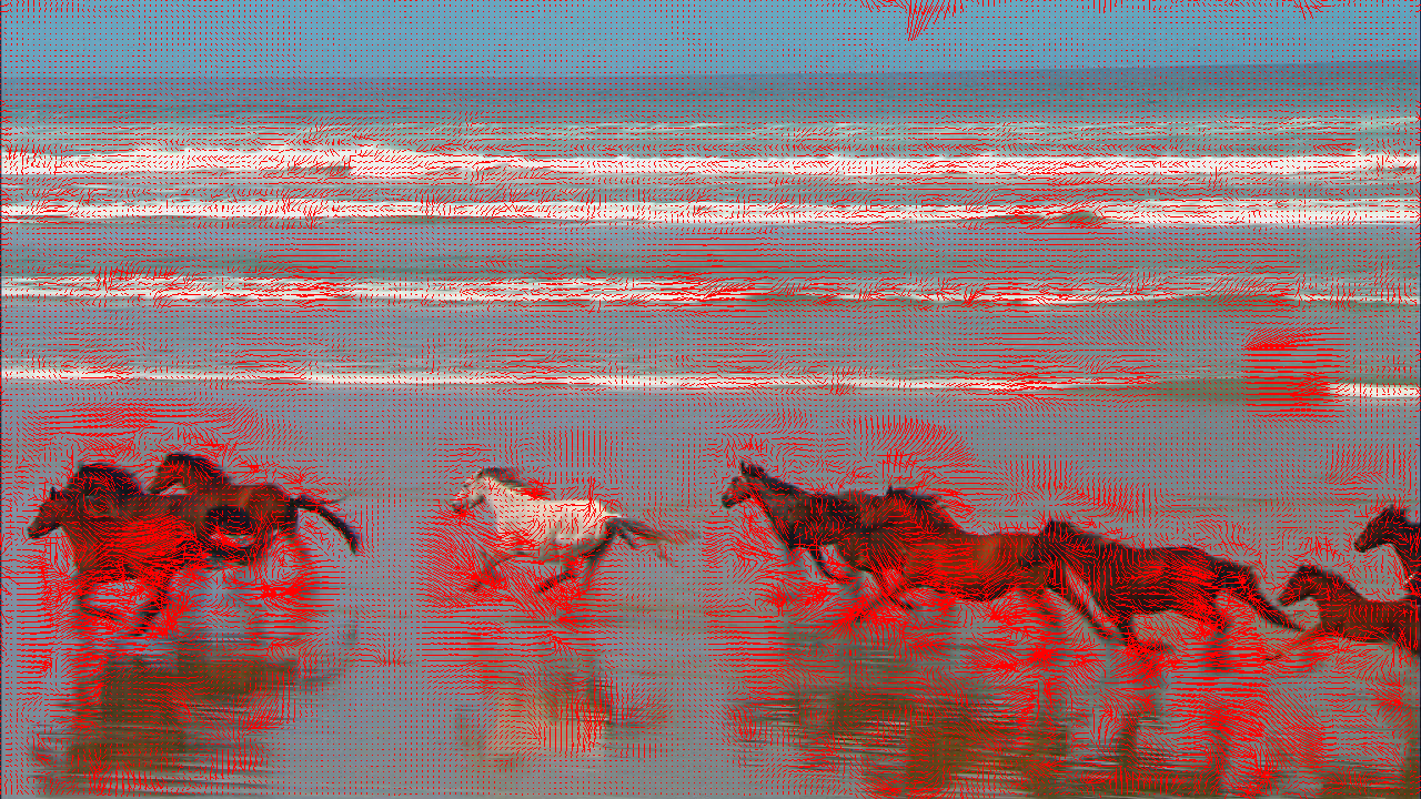
2019-12-27Advancements in computer vision research have revolutionized the way machines perceive their environment by leveraging techniques like object detection for recognizing objects belonging to a specific class and semantic segmentation for pixel-level classification. However, when it comes to real-time video processing, most implementations of these techniques only consider the spatial relationships of objects within the same frame (x,y) while ignoring the temporal aspect (t). This means that each frame is evaluated independently, without any correlation to previous or future frames. But, what if we require the relationship between consecutive frames? For example, what if we want to track the movement of vehicles across frames to estimate their current speed and predict their position in the next frame?
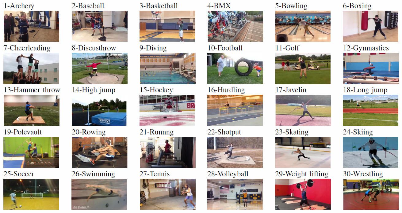
Alternatively, what if we require information on human pose relationships between consecutive frames to recognize human actions such as archery, baseball, and basketball?
In this tutorial, we will learn what Optical Flow is, how to implement its two main variants (sparse and dense), and also get a big picture of more recent approaches involving deep learning and promising future directions.
What is optical flow?
Let us begin with a high-level understanding of optical flow. Optical flow is the motion of objects between consecutive frames of the sequence, caused by the relative movement between the object and the camera. The problem of optical flow may be expressed as:
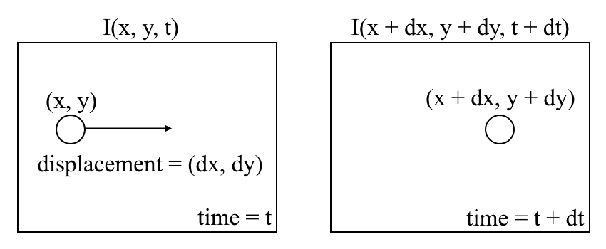
where between consecutive frames, we can express the image intensity (I) as a function of space (x,y) and time (t). In other words, if we take the first image I(x,y,t) and move its pixels by (dx,dy) over t time, we obtain the new image I(x+dx,y+dy,t+dt).
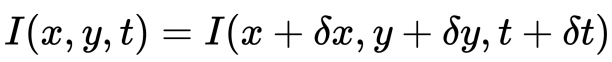
First, we assume that the pixel intensities of an object are constant between consecutive frames.
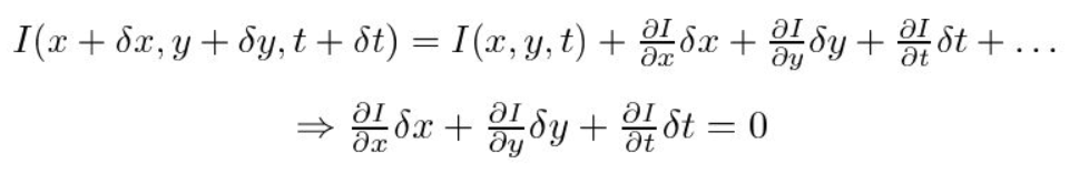
Second, we take the Taylor Series Approximation of the RHS and remove common terms.
Third, we divide by dt to derive the optical flow equation:
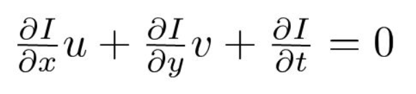
where u=dx/dt and v=dy/dt.
dI/dx, dI/dy, and dI/dt are the image gradients along the horizontal axis, the vertical axis, and time. Hence, we conclude with the problem of optical flow, that is, solving u(dx/dt) and v(dy/dt) to determine movement over time. You may notice that we cannot directly solve the optical flow equation for u and v since there is only one equation for two unknown variables. We will implement some methods such as the Lucas-Kanade method to address this issue.
Sparse vs Dense Optical Flow
Sparse optical flow gives the flow vectors of some “interesting features” (say a few pixels depicting the edges or corners of an object) within the frame while Dense optical flow, which gives the flow vectors of the entire frame (all pixels) – up to one flow vector per pixel. As you would’ve guessed, Dense optical flow has higher accuracy at the cost of being slow/computationally expensive.
Implementing Sparse Optical Flow
Sparse optical flow selects a sparse feature set of pixels (e.g. interesting features such as edges and corners) to track its velocity vectors (motion). The extracted features are passed in the optical flow function from frame to frame to ensure that the same points are being tracked. There are various implementations of sparse optical flow, including the Lucas–Kanade method, the Horn–Schunck method, the Buxton–Buxton method, and more. We will be using the Lucas-Kanade method with OpenCV, an open-source library of computer vision algorithms, for implementation.
1. Setting up your environment
If you do not already have OpenCV installed, open Terminal and run:
pip install opencv-python
Now, clone the tutorial repository by running:
git clone https://github.com/chuanenlin/optical-flow.git
Next, open sparse-starter.py with your text editor. We will be writing all of the code in this Python file.
2. Configuring OpenCV to read a video and setting up parameters
import cv2 as cv
import numpy as np

# Parameters for Shi-Tomasi corner detection
feature_params = dict(maxCorners = 300, qualityLevel = 0.2, minDistance = 2, blockSize = 7)
# Parameters for Lucas-Kanade optical flow
lk_params = dict(winSize = (15,15), maxLevel = 2, criteria = (cv.TERM_CRITERIA_EPS | cv.TERM_CRITERIA_COUNT, 10, 0.03))
# The video feed is read in as a VideoCapture object
cap = cv.VideoCapture("shibuya.mp4")
# Variable for color to draw optical flow track
color = (0, 255, 0)
# ret = a boolean return value from getting the frame, first_frame = the first frame in the entire video sequence
ret, first_frame = cap.read()

while(cap.isOpened()):
    # ret = a boolean return value from getting the frame, frame = the current frame being projected in the video
    ret, frame = cap.read()
    # Frames are read by intervals of 10 milliseconds. The programs breaks out of the while loop when the user presses the 'q' key
    if cv.waitKey(10) & 0xFF == ord('q'):
        break
# The following frees up resources and closes all windows
cap.release()
cv.destroyAllWindows()
3. Grayscaling
import cv2 as cv
import numpy as np

# Parameters for Shi-Tomasi corner detection
# feature_params = dict(maxCorners = 300, qualityLevel = 0.2, minDistance = 2, blockSize = 7)
# Parameters for Lucas-Kanade optical flow
# lk_params = dict(winSize = (15,15), maxLevel = 2, criteria = (cv.TERM_CRITERIA_EPS | cv.TERM_CRITERIA_COUNT, 10, 0.03))
# The video feed is read in as a VideoCapture object
# cap = cv.VideoCapture("shibuya.mp4")
# Variable for color to draw optical flow track
# color = (0, 255, 0)
# ret = a boolean return value from getting the frame, first_frame = the first frame in the entire video sequence
# ret, first_frame = cap.read()
# Converts frame to grayscale because we only need the luminance channel for detecting edges - less computationally expensive
prev_gray = cv.cvtColor(first_frame, cv.COLOR_BGR2GRAY)

# while(cap.isOpened()):
    # ret = a boolean return value from getting the frame, frame = the current frame being projected in the video
    # ret, frame = cap.read()
    # Converts each frame to grayscale - we previously only converted the first frame to grayscale
    gray = cv.cvtColor(frame, cv.COLOR_BGR2GRAY)
    # Visualizes checkpoint 2
    cv.imshow("grayscale", gray)
    # Updates previous frame
    prev_gray = gray.copy()
    # Frames are read by intervals of 10 milliseconds. The programs breaks out of the while loop when the user presses the 'q' key
    # if cv.waitKey(10) & 0xFF == ord('q'):
        # break
# The following frees up resources and closes all windows
# cap.release()
# cv.destroyAllWindows()
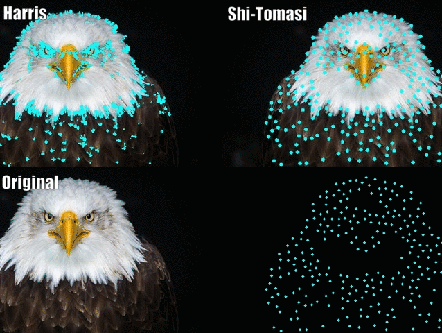
4. Shi-Tomasi Corner Detector – selecting the pixels to track
For the implementation of sparse optical flow, we only track the motion of a feature set of pixels. Features in images are points of interest that present rich image content information. For example, such features may be points in the image that are invariant to translation, scale, rotation, and intensity changes such as corners.
The Shi-Tomasi Corner Detector is very similar to the popular Harris Corner Detector which can be implemented by the following three procedures:
- Determine windows (small image patches) with large gradients (variations in image intensity) when translated in both xx and yy directions.
- For each window, compute a score R.
- Depending on the value of R, each window is classified as a flat, edge, or corner.
If you would like to know more about a step-by-step mathematical explanation of the Harris Corner Detector, feel free to go through these slides. Shi and Tomasi later made a small but effective modification to the Harris Corner Detector in their paper Good Features to Track.
The modification is to the equation in which the score R is calculated. In the Harris Corner Detector, the scoring function is given by:

Instead, Shi-Tomasi proposed the scoring function as:
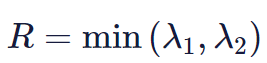
which basically means if RR is greater than a threshold, it is classified as a corner. The following compares the scoring functions of Harris (left) and Shi-Tomasi (right) in λ1−λ2 space.
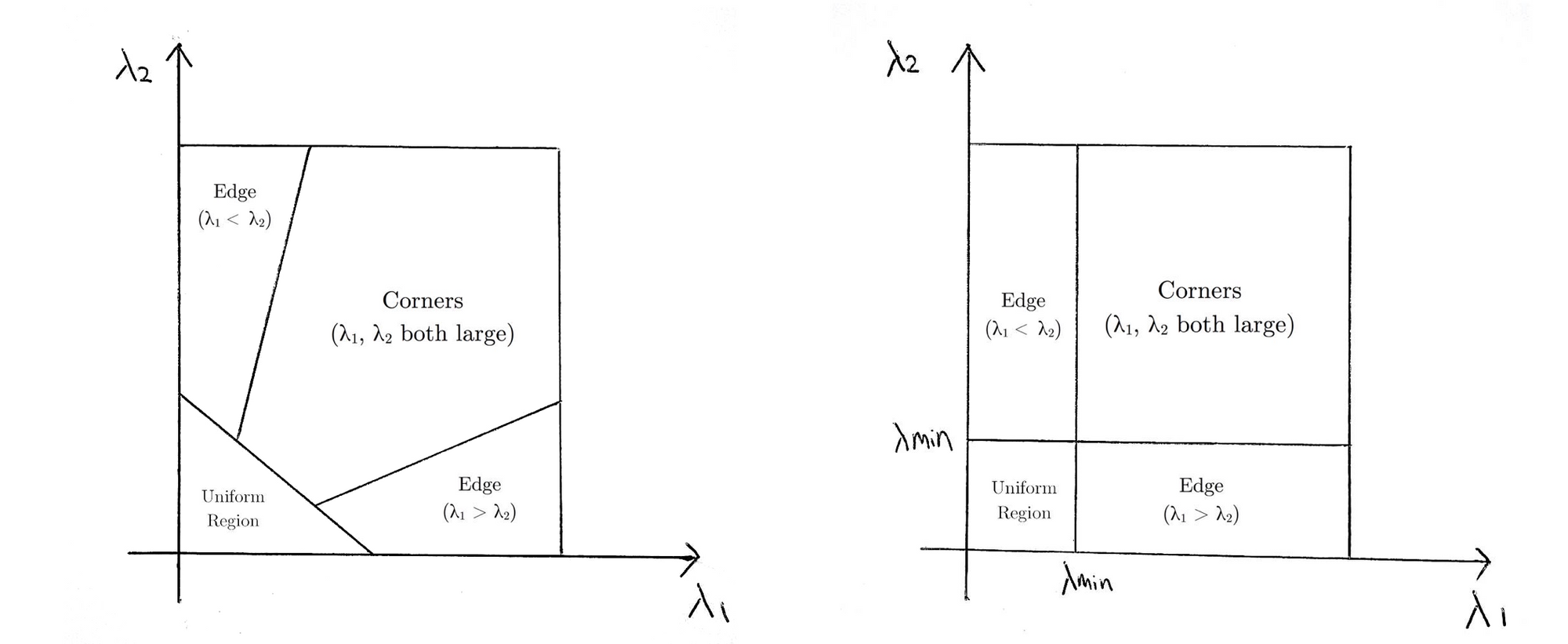
For Shi-Tomasi, only when λ1 and λ2 are above a minimum threshold λminλmin is the window classified as a corner.
The documentation of OpenCV’s implementation of Shi-Tomasi via goodFeaturesToTrack() may be found here.
import cv2 as cv
import numpy as np

# Parameters for Shi-Tomasi corner detection
# feature_params = dict(maxCorners = 300, qualityLevel = 0.2, minDistance = 2, blockSize = 7)
# Parameters for Lucas-Kanade optical flow
# lk_params = dict(winSize = (15,15), maxLevel = 2, criteria = (cv.TERM_CRITERIA_EPS | cv.TERM_CRITERIA_COUNT, 10, 0.03))
# The video feed is read in as a VideoCapture object
# cap = cv.VideoCapture("shibuya.mp4")
# Variable for color to draw optical flow track
# color = (0, 255, 0)
# ret = a boolean return value from getting the frame, first_frame = the first frame in the entire video sequence
# ret, first_frame = cap.read()
# Converts frame to grayscale because we only need the luminance channel for detecting edges - less computationally expensive
# prev_gray = cv.cvtColor(first_frame, cv.COLOR_BGR2GRAY)
# Finds the strongest corners in the first frame by Shi-Tomasi method - we will track the optical flow for these corners
# https://docs.opencv.org/3.0-beta/modules/imgproc/doc/feature_detection.html#goodfeaturestotrack
prev = cv.goodFeaturesToTrack(prev_gray, mask = None, **feature_params)

# while(cap.isOpened()):
    # ret = a boolean return value from getting the frame, frame = the current frame being projected in the video
    # ret, frame = cap.read()
    # Converts each frame to grayscale - we previously only converted the first frame to grayscale
    # gray = cv.cvtColor(frame, cv.COLOR_BGR2GRAY)
    # Updates previous frame
    # prev_gray = gray.copy()
    # Frames are read by intervals of 10 milliseconds. The programs breaks out of the while loop when the user presses the 'q' key
    # if cv.waitKey(10) & 0xFF == ord('q'):
        # break
# The following frees up resources and closes all windows
# cap.release()
# cv.destroyAllWindows()
Tracking Specific Objects
There may be scenarios where you want to only track a specific object of interest (say tracking a certain person) or one category of objects (like all 2 wheeled vehicles in traffic). You can easily modify the code to track the pixels of the object(s) you want by changing the prev variable.
You can also combine Object Detection with this method to only estimate the flow of pixels within the detected bounding boxes. This way you can track all objects of a particular type/category in the video.
5. Lucas-Kanade: Sparse Optical Flow
Lucas and Kanade proposed an effective technique to estimate the motion of interesting features by comparing two consecutive frames in their paper An Iterative Image Registration Technique with an Application to Stereo Vision. The Lucas-Kanade method works under the following assumptions:
- Two consecutive frames are separated by a small-time increment (dt) such that objects are not displaced significantly (in other words, the method works best with slow-moving objects).
- A frame portrays a “natural” scene with textured objects exhibiting shades of gray that change smoothly.
First, under these assumptions, we can take a small 3×3 window (neighborhood) around the features detected by Shi-Tomasi and assume that all nine points have the same motion.
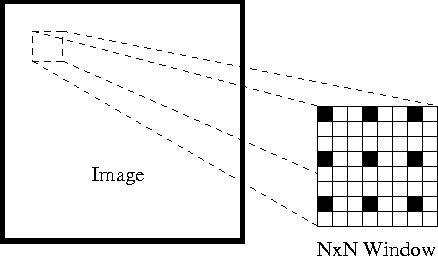
This may be represented as
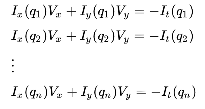
where q1,q2,…,qn denote the pixels inside the window (e.g. n = 9 for a 3×3 window) and Ix(qi), Iy(qi), and It(qi) denote the partial derivatives of image II with respect to the position (x,y) and time tt, for pixel qi at the current time.
This is just the Optical Flow Equation for each of the n pixels.
The set of equations may be represented in the following matrix form where Av=b:
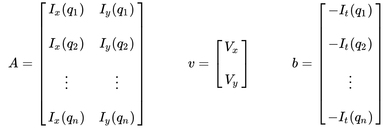
Take note that previously (see “What is optical flow?” section), we faced the issue of having to solve for two unknown variables with one equation. We now face having to solve for two unknowns (Vx and Vy) with nine equations, which is over-determined.
Second, to address the over-determined issue, we apply a least-squares fitting to obtain the following two-equation-two-unknown problem:
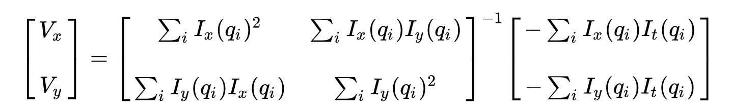
where Vx=u=dx/dt denotes the movement of xx over time and Vy=v=dy/dt denotes the movement of y over time. Solving the two variables completes the optical flow problem.
In a nutshell, we identify some interesting features to track and iteratively compute the optical flow vectors of these points. However, adopting the Lucas-Kanade method only works for small movements (from our initial assumption) and fails when there is a large motion. Therefore, the OpenCV implementation of the Lucas-Kanade method adopts pyramids.
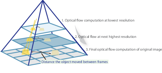
In a high-level view, small motions are neglected as we go up the pyramid and large motions are reduced to small motions – we compute optical flow along with scale. A comprehensive mathematical explanation of OpenCV’s implementation may be found in Bouguet’s notes and the documentation of OpenCV’s implementation of the Lucas-Kanade method via calcOpticalFlowPyrLK() may be found here.
import cv2 as cv
import numpy as np

# Parameters for Shi-Tomasi corner detection
# feature_params = dict(maxCorners = 300, qualityLevel = 0.2, minDistance = 2, blockSize = 7)
# Parameters for Lucas-Kanade optical flow
# lk_params = dict(winSize = (15,15), maxLevel = 2, criteria = (cv.TERM_CRITERIA_EPS | cv.TERM_CRITERIA_COUNT, 10, 0.03))
# The video feed is read in as a VideoCapture object
# cap = cv.VideoCapture("shibuya.mp4")
# Variable for color to draw optical flow track
# color = (0, 255, 0)
# ret = a boolean return value from getting the frame, first_frame = the first frame in the entire video sequence
# ret, first_frame = cap.read()
# Converts frame to grayscale because we only need the luminance channel for detecting edges - less computationally expensive
# prev_gray = cv.cvtColor(first_frame, cv.COLOR_BGR2GRAY)
# Finds the strongest corners in the first frame by Shi-Tomasi method - we will track the optical flow for these corners
# https://docs.opencv.org/3.0-beta/modules/imgproc/doc/feature_detection.html#goodfeaturestotrack
# prev = cv.goodFeaturesToTrack(prev_gray, mask = None, **feature_params)

# while(cap.isOpened()):
    # ret = a boolean return value from getting the frame, frame = the current frame being projected in the video
    # ret, frame = cap.read()
    # Converts each frame to grayscale - we previously only converted the first frame to grayscale
    # gray = cv.cvtColor(frame, cv.COLOR_BGR2GRAY)
    # Calculates sparse optical flow by Lucas-Kanade method
    # https://docs.opencv.org/3.0-beta/modules/video/doc/motion_analysis_and_object_tracking.html#calcopticalflowpyrlk
    next, status, error = cv.calcOpticalFlowPyrLK(prev_gray, gray, prev, None, **lk_params)
    # Selects good feature points for previous position
    good_old = prev[status == 1]
    # Selects good feature points for next position
    good_new = next[status == 1]
    # Updates previous frame
    # prev_gray = gray.copy()
    # Updates previous good feature points
    prev = good_new.reshape(-1, 1, 2)
    # Frames are read by intervals of 10 milliseconds. The programs breaks out of the while loop when the user presses the 'q' key
    # if cv.waitKey(10) & 0xFF == ord('q'):
        # break
# The following frees up resources and closes all windows
# cap.release()
# cv.destroyAllWindows()
6. Visualizing
import cv2 as cv
import numpy as np

# Parameters for Shi-Tomasi corner detection
# feature_params = dict(maxCorners = 300, qualityLevel = 0.2, minDistance = 2, blockSize = 7)
# Parameters for Lucas-Kanade optical flow
# lk_params = dict(winSize = (15,15), maxLevel = 2, criteria = (cv.TERM_CRITERIA_EPS | cv.TERM_CRITERIA_COUNT, 10, 0.03))
# The video feed is read in as a VideoCapture object
# cap = cv.VideoCapture("shibuya.mp4")
# Variable for color to draw optical flow track
# color = (0, 255, 0)
# ret = a boolean return value from getting the frame, first_frame = the first frame in the entire video sequence
# ret, first_frame = cap.read()
# Converts frame to grayscale because we only need the luminance channel for detecting edges - less computationally expensive
# prev_gray = cv.cvtColor(first_frame, cv.COLOR_BGR2GRAY)
# Finds the strongest corners in the first frame by Shi-Tomasi method - we will track the optical flow for these corners
# https://docs.opencv.org/3.0-beta/modules/imgproc/doc/feature_detection.html#goodfeaturestotrack
# prev = cv.goodFeaturesToTrack(prev_gray, mask = None, **feature_params)
# Creates an image filled with zero intensities with the same dimensions as the frame - for later drawing purposes
mask = np.zeros_like(first_frame)

# while(cap.isOpened()):
    # ret = a boolean return value from getting the frame, frame = the current frame being projected in the video
    # ret, frame = cap.read()
    # Converts each frame to grayscale - we previously only converted the first frame to grayscale
    # gray = cv.cvtColor(frame, cv.COLOR_BGR2GRAY)
    # Calculates sparse optical flow by Lucas-Kanade method
    # https://docs.opencv.org/3.0-beta/modules/video/doc/motion_analysis_and_object_tracking.html#calcopticalflowpyrlk
    # next, status, error = cv.calcOpticalFlowPyrLK(prev_gray, gray, prev, None, **lk_params)
    # Selects good feature points for previous position
    # good_old = prev[status == 1]
    # Selects good feature points for next position
    # good_new = next[status == 1]
    # Draws the optical flow tracks
    for i, (new, old) in enumerate(zip(good_new, good_old)):
        # Returns a contiguous flattened array as (x, y) coordinates for new point
        a, b = new.ravel()
        # Returns a contiguous flattened array as (x, y) coordinates for old point
        c, d = old.ravel()
        # Draws line between new and old position with green color and 2 thickness
        mask = cv.line(mask, (a, b), (c, d), color, 2)
        # Draws filled circle (thickness of -1) at new position with green color and radius of 3
        frame = cv.circle(frame, (a, b), 3, color, -1)
    # Overlays the optical flow tracks on the original frame
    output = cv.add(frame, mask)
    # Updates previous frame
    # prev_gray = gray.copy()
    # Updates previous good feature points
    # prev = good_new.reshape(-1, 1, 2)
    # Opens a new window and displays the output frame
    cv.imshow("sparse optical flow", output)
    # Frames are read by intervals of 10 milliseconds. The programs breaks out of the while loop when the user presses the 'q' key
    # if cv.waitKey(10) & 0xFF == ord('q'):
        # break
# The following frees up resources and closes all windows
# cap.release()
# cv.destroyAllWindows()
And that’s it! Open Terminal and run
python sparse-starter.py
to test your sparse optical flow implementation. 👏
In case you have missed any code, the full code can be found in sparse-solution.py.
Implementing Dense Optical Flow
We’ve previously computed the optical flow for a sparse feature set of pixels. Dense optical flow attempts to compute the optical flow vector for every pixel of each frame. While such computation may be slower, it gives a more accurate result and a denser result suitable for applications such as learning structure from motion and video segmentation. There are various implementations of dense optical flow. We will be using the Farneback method, one of the most popular implementations, with using OpenCV, an open-source library of computer vision algorithms, for implementation.
1. Setting up your environment
If you have not done so already, please follow Step 1 of implementing sparse optical flow to set up your environment.
Next, open dense-starter.py with your text editor. We will be writing all of the code in this Python file.
2. Configuring OpenCV to read a video
import cv2 as cv
import numpy as np

# The video feed is read in as a VideoCapture object
cap = cv.VideoCapture("shibuya.mp4")
# ret = a boolean return value from getting the frame, first_frame = the first frame in the entire video sequence
ret, first_frame = cap.read()

while(cap.isOpened()):
    # ret = a boolean return value from getting the frame, frame = the current frame being projected in the video
    ret, frame = cap.read()
    # Opens a new window and displays the input frame
    cv.imshow("input", frame)
    # Frames are read by intervals of 1 millisecond. The programs breaks out of the while loop when the user presses the 'q' key
    if cv.waitKey(1) & 0xFF == ord('q'):
        break
# The following frees up resources and closes all windows
cap.release()
cv.destroyAllWindows()
3. Grayscaling
import cv2 as cv
import numpy as np

# The video feed is read in as a VideoCapture object
# cap = cv.VideoCapture("shibuya.mp4")
# ret = a boolean return value from getting the frame, first_frame = the first frame in the entire video sequence
# ret, first_frame = cap.read()
# Converts frame to grayscale because we only need the luminance channel for detecting edges - less computationally expensive
prev_gray = cv.cvtColor(first_frame, cv.COLOR_BGR2GRAY)

# while(cap.isOpened()):
    # ret = a boolean return value from getting the frame, frame = the current frame being projected in the video
    # ret, frame = cap.read()
    # Opens a new window and displays the input frame
    # cv.imshow("input", frame)
    # Converts each frame to grayscale - we previously only converted the first frame to grayscale
    gray = cv.cvtColor(frame, cv.COLOR_BGR2GRAY)
    # Visualizes checkpoint 2
    cv.imshow("grayscale", gray)
    # Updates previous frame
    prev_gray = gray
    # Frames are read by intervals of 1 millisecond. The programs breaks out of the while loop when the user presses the 'q' key
    # if cv.waitKey(1) & 0xFF == ord('q'):
        # break
# The following frees up resources and closes all windows
# cap.release()
# cv.destroyAllWindows()
4. Farneback Optical Flow
Gunnar Farneback proposed an effective technique to estimate the motion of interesting features by comparing two consecutive frames in his paper Two-Frame Motion Estimation Based on Polynomial Expansion.
First, the method approximates the windows (see Lucas Kanade section of sparse optical flow implementation for more details) of image frames by quadratic polynomials through polynomial expansion transform. Second, by observing how the polynomial transforms under translation (motion), a method to estimate displacement fields from polynomial expansion coefficients is defined. After a series of refinements, dense optical flow is computed. Farneback’s paper is fairly concise and straightforward to follow so I highly recommend going through the paper if you would like a greater understanding of its mathematical derivation.
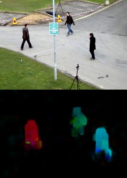
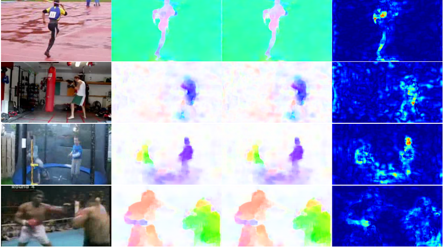
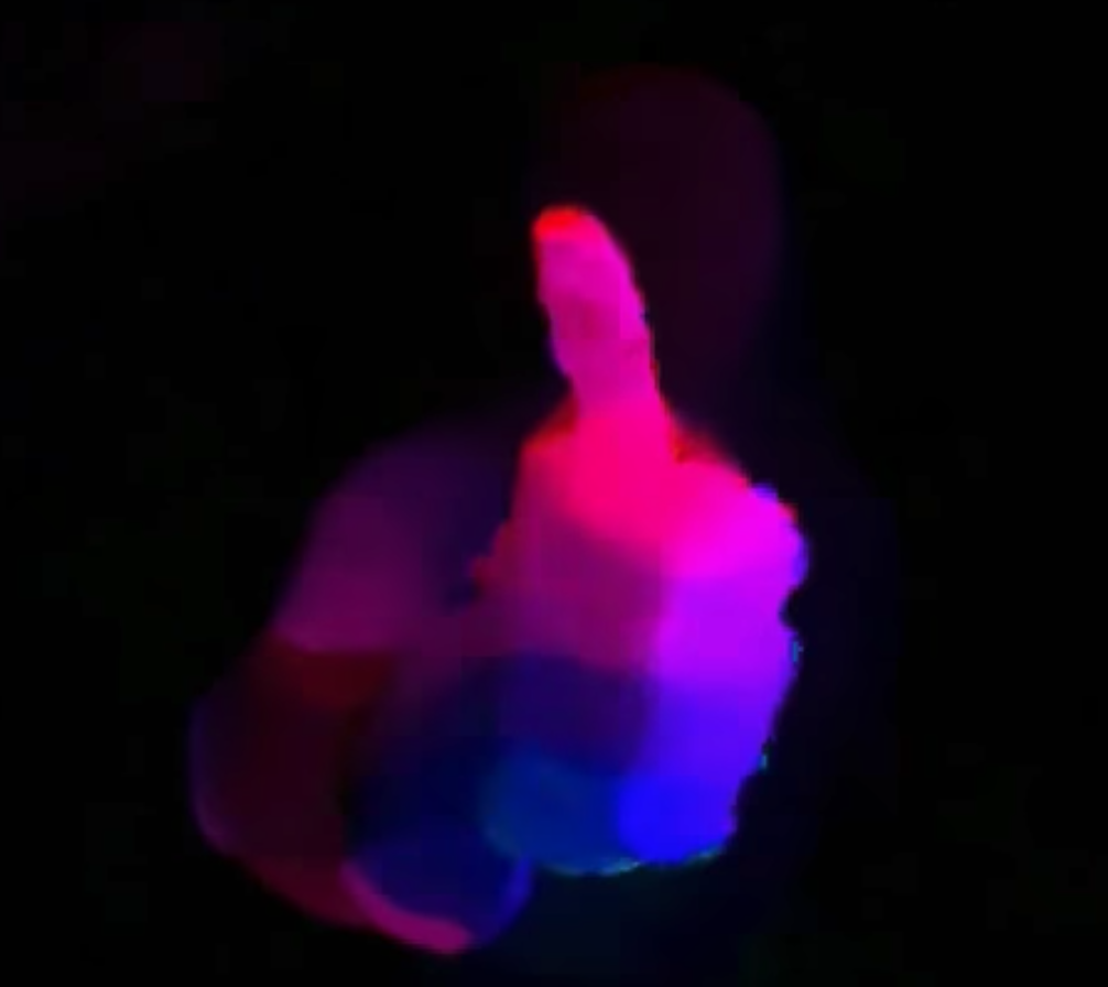
For OpenCV’s implementation, it computes the magnitude and direction of optical flow from a 2-channel array of flow vectors (dx/dt,dy/dt), the optical flow problem. It then visualizes the angle (direction) of flow by hue and the distance (magnitude) of flow by the value of HSV color representation. The strength of HSV is always set to a maximum of 255 for optimal visibility. The documentation of OpenCV’s implementation of the Farneback method via calcOpticalFlowFarneback() may be found here.
import cv2 as cv
import numpy as np

# The video feed is read in as a VideoCapture object
# cap = cv.VideoCapture("shibuya.mp4")
# ret = a boolean return value from getting the frame, first_frame = the first frame in the entire video sequence
# ret, first_frame = cap.read()
# Converts frame to grayscale because we only need the luminance channel for detecting edges - less computationally expensive
# prev_gray = cv.cvtColor(first_frame, cv.COLOR_BGR2GRAY)

# while(cap.isOpened()):
    # ret = a boolean return value from getting the frame, frame = the current frame being projected in the video
    # ret, frame = cap.read()
    # Opens a new window and displays the input frame
    # cv.imshow("input", frame)
    # Converts each frame to grayscale - we previously only converted the first frame to grayscale
    # gray = cv.cvtColor(frame, cv.COLOR_BGR2GRAY)
    # Calculates dense optical flow by Farneback method
    # https://docs.opencv.org/3.0-beta/modules/video/doc/motion_analysis_and_object_tracking.html#calcopticalflowfarneback
    flow = cv.calcOpticalFlowFarneback(prev_gray, gray, None, 0.5, 3, 15, 3, 5, 1.2, 0)
    # Updates previous frame
    # prev_gray = gray
    # Frames are read by intervals of 1 millisecond. The programs breaks out of the while loop when the user presses the 'q' key
    # if cv.waitKey(1) & 0xFF == ord('q'):
        # break
# The following frees up resources and closes all windows
# cap.release()
# cv.destroyAllWindows()
5. Visualizing
import cv2 as cv
import numpy as np

# The video feed is read in as a VideoCapture object
# cap = cv.VideoCapture("shibuya.mp4")
# ret = a boolean return value from getting the frame, first_frame = the first frame in the entire video sequence
# ret, first_frame = cap.read()
# Converts frame to grayscale because we only need the luminance channel for detecting edges - less computationally expensive
# prev_gray = cv.cvtColor(first_frame, cv.COLOR_BGR2GRAY)
# Creates an image filled with zero intensities with the same dimensions as the frame
mask = np.zeros_like(first_frame)
# Sets image saturation to maximum
mask[..., 1] = 255

# while(cap.isOpened()):
    # ret = a boolean return value from getting the frame, frame = the current frame being projected in the video
    # ret, frame = cap.read()
    # Opens a new window and displays the input frame
    # cv.imshow("input", frame)
    # Converts each frame to grayscale - we previously only converted the first frame to grayscale
    # gray = cv.cvtColor(frame, cv.COLOR_BGR2GRAY)
    # Calculates dense optical flow by Farneback method
    # https://docs.opencv.org/3.0-beta/modules/video/doc/motion_analysis_and_object_tracking.html#calcopticalflowfarneback
    # flow = cv.calcOpticalFlowFarneback(prev_gray, gray, None, 0.5, 3, 15, 3, 5, 1.2, 0)
    # Computes the magnitude and angle of the 2D vectors
    magnitude, angle = cv.cartToPolar(flow[..., 0], flow[..., 1])
    # Sets image hue according to the optical flow direction
    mask[..., 0] = angle * 180 / np.pi / 2
    # Sets image value according to the optical flow magnitude (normalized)
    mask[..., 2] = cv.normalize(magnitude, None, 0, 255, cv.NORM_MINMAX)
    # Converts HSV to RGB (BGR) color representation
    rgb = cv.cvtColor(mask, cv.COLOR_HSV2BGR)
    # Opens a new window and displays the output frame
    cv.imshow("dense optical flow", rgb)
    # Updates previous frame
    # prev_gray = gray
    # Frames are read by intervals of 1 millisecond. The programs breaks out of the while loop when the user presses the 'q' key
    # if cv.waitKey(1) & 0xFF == ord('q'):
        # break
# The following frees up resources and closes all windows
# cap.release()
# cv.destroyAllWindows()
And that’s it! Open Terminal and run
python dense-starter.py
to test your dense optical flow implementation.
In case you have missed any code, the full code can be found in dense-solution.py.
Optical Flow using Deep Learning
While the problem of optical flow has historically been an optimization problem, recent approaches by applying deep learning have shown impressive results. Generally, such approaches take two video frames as input to output the optical flow (color-coded image), which may be expressed as:

where u is the motion in the x direction, v is the motion in the yy direction, and f is a neural network that takes in two consecutive frames I_(t−1) (frame at time = t−1) and I_t (frame at time = t) as input.
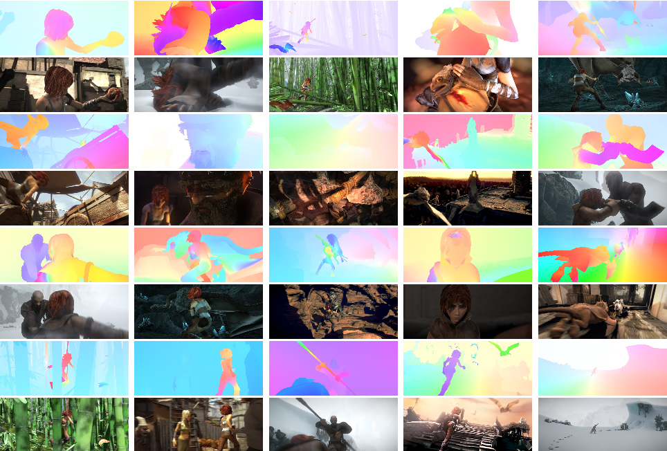
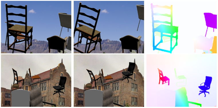
Computing optical flow with deep neural networks requires large amounts of training data which is particularly hard to obtain. This is because labeling video footage for optical flow requires accurately figuring out the exact motion of every point of an image to subpixel accuracy. To address the issue of labeling training data, researchers used computer graphics to simulate massive realistic worlds. Since the worlds are generated by instruction, the motion of each and every point of an image in a video sequence is known. Some examples of such include MPI-Sintel, an open-source CGI movie with optical flow labeling rendered for various sequences, and Flying Chairs, a dataset of many chairs flying across random backgrounds also with optical flow labeling.
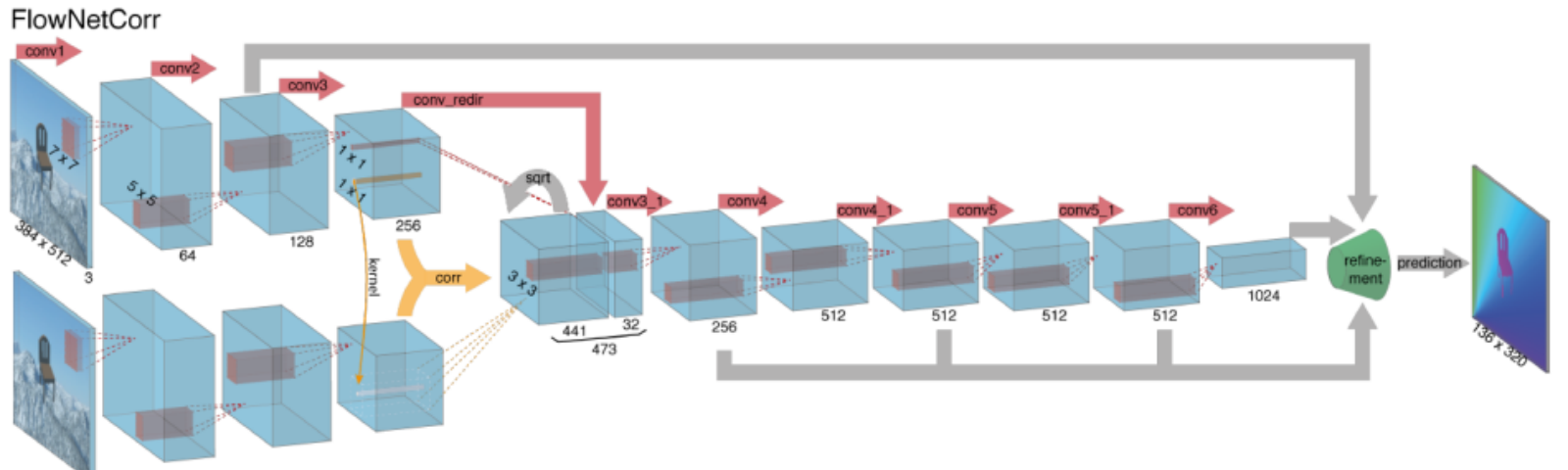
Solving optical flow problems with deep learning is an extremely hot topic at the moment, with variants of FlowNet, SPyNet, PWC-Net, and more each outperforming one another on various benchmarks.
Optical Flow application: Semantic Segmentation
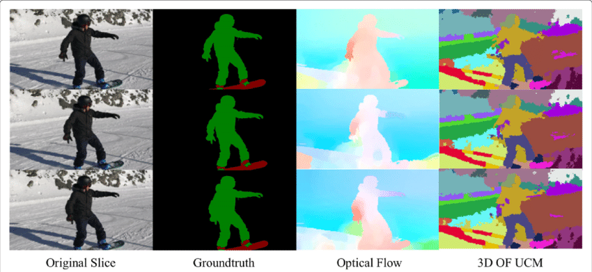
The optical flow field is a vast mine of information for the observed scene. As the techniques of accurately determining optical flow improve, it is interesting to see applications of optical flow in junctions with several other fundamental computer vision tasks. For example, the task of semantic segmentation is to divide an image into a series of regions corresponding to unique object classes yet closely placed objects with identical textures are often difficult for single frame segmentation techniques. If the objects are placed separately, however, the distinct motions of the objects may be highly helpful where discontinuity in the dense optical flow field corresponds to boundaries between objects.
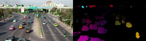
Optical Flow application: Object Detection & Tracking
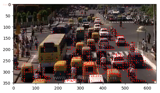
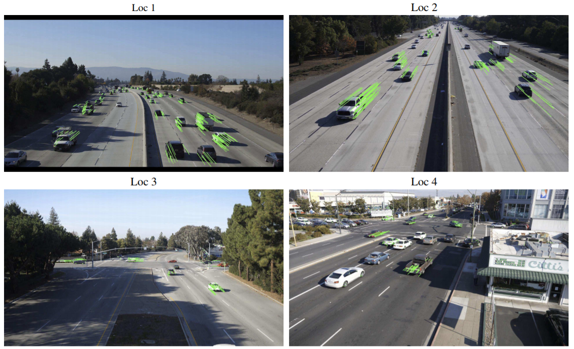
Another promising application of optical flow may be with object detection and tracking or, in a high-level form, towards building real-time vehicle tracking and traffic analysis systems. Since sparse optical flow utilizes tracking of points of interest, such real-time systems may be performed by feature-based optical flow techniques from either from a stationary camera or cameras attached to vehicles.
Conclusion
Fundamentally, optical flow vectors function as input to a myriad of higher-level tasks requiring scene understanding of video sequences while these tasks may further act as building blocks to yet more complex systems such as facial expression analysis, autonomous vehicle navigation, and much more. Novel applications for optical flow yet to be discovered are limited only by the ingenuity of its designers.
References:
https://nanonets.com/blog/optical-flow/
3 Comments
Hi, when you say “You can easily modify the code to track the pixels of the object(s) you want by changing the prev variable.” how do I do this?
i have more than 9000 frames from River Videos that captured by UAV, i want Ensemble some CNN Models for estimating River flow velocity using FlowNet,PWC-Net and … Models.
Please guide me for making Ensemble model by python.
Why in the dense optical flow, when converting the angle to degrees, it is divided by 2? I don’t get to understand why
mask[…, 0] = angle * 180 / np.pi / 2