Machine Learning Interview: Basics

42 mins read

In this post, I will provide the answers to the questions for the online ML interview book.

1) Explain supervised, unsupervised, weakly supervised, semi-supervised, and active learning.

Supervised Learning: Supervised learning is a type of machine learning where the algorithm is trained using labeled data. The labeled data consists of input and output pairs, where the algorithm learns to map inputs to outputs. The aim of supervised learning is to build a model that can accurately predict the output for new unseen input data.
Unsupervised Learning: Unsupervised learning is a type of machine learning where the algorithm is trained using unlabeled data. In unsupervised learning, the algorithm is left to find patterns, structures, and relationships in the data on its own. The goal of unsupervised learning is to uncover hidden patterns and groupings within the data.
Weakly Supervised Learning:

The insight behind weak supervision is that people rely on heuristics, which can be developed with subject matter expertise, to label data. For example, a doctor might use the following heuristics to decide whether a patient’s case should be prioritized as
emergent:
If the nurse’s note mentions a serious condition like pneumonia, the patient’s case should be given priority consideration.

Weak learning libraries like Snorkel are built around the concept of a Labeling Function (LF): a function that encodes heuristics. The preceding heuristics can be expressed by the following function:
def labeling_function(note):
if “pneumonia” in note:
return “EMERGENT”

LFs can encode many different types of heuristics. Here are some of them:
Keyword heuristic
Such as the preceding example
Regular expressions
Such as if the note matches or fails to match a certain regular expression
Database lookup
Such as if the note contains the disease listed in the dangerous disease list
The outputs of other models
Such as if an existing system classifies this as EMERGENT
After you’ve written LFs, you can apply them to the samples you want to label. Because LFs encode heuristics, and heuristics are noisy, labels produced by LFs are noisy. Multiple LFs might apply to the same data examples, and they might give conflicting labels. One function might think a nurse’s note is EMERGENT but another function might think it’s not. One heuristic might be much more accurate than another heuristic, which you might not know because you don’t have ground truth labels to compare them to. It’s important to combine, denoise, and reweight all LFs to get a set of most likely to be correct labels.

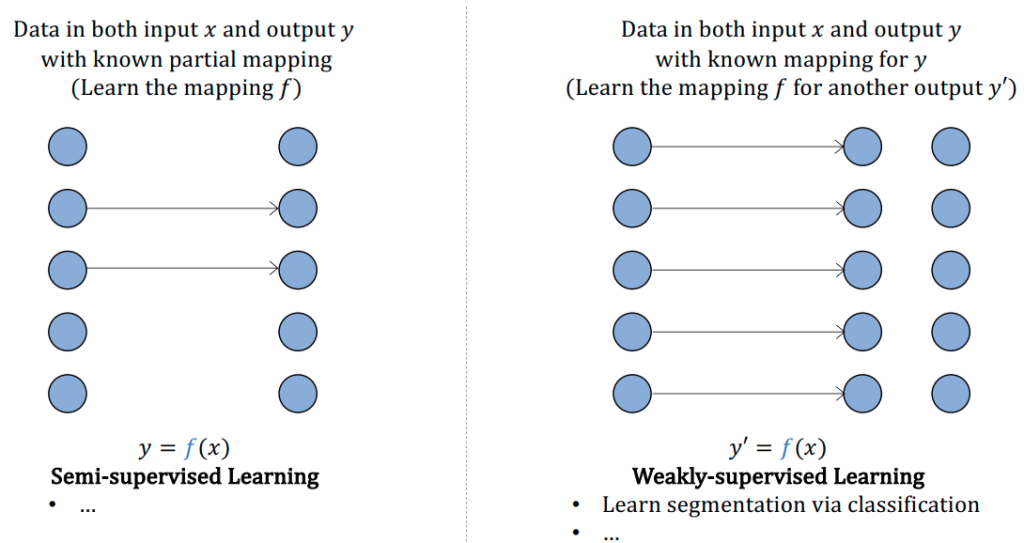
Semi-Supervised Learning: Semi-supervised learning is a type of machine learning where the algorithm is trained using a combination of labeled and unlabeled data. The labeled data is used to build a model that can accurately predict the output for new unseen input data, while the unlabeled data is used to improve the model’s generalization ability and to learn more about the underlying structure of the data.

If weak supervision leverages heuristics to obtain noisy labels, semi-supervision leverages structural assumptions to generate new labels based on a small set of initial labels. Unlike weak supervision, semi-supervision requires an initial set of labels.

A classic semi-supervision method is self-training. You start by training a model on your existing set of labeled data and use this model to make predictions for unlabeled samples. Assuming that predictions with high raw probability scores are correct, you add the labels predicted with high probability to your training set and train a new model on this expanded training set. This goes on until you’re happy with your model performance.
Another semi-supervision method assumes that data samples that share similar characteristics share the same labels. The similarity might be obvious, such as in the task of classifying the topic of Twitter hashtags. You can start by labeling the hashtag
“#AI” as Computer Science. Assuming that hashtags that appear in the same tweet or profile are likely about the same topic. You can also label the hashtags “#ML” and “#BigData” as Computer Science.

Active Learning: Active learning is a type of machine learning where the algorithm is allowed to interactively query the user or expert to obtain the desired output labels for a subset of the data. The aim of active learning is to reduce the amount of labeled data needed to train an accurate model, by selecting the most informative and relevant samples to be labeled. This can save time and resources in situations where labeling data is expensive or time-consuming.

Active learning is a method for improving the efficiency of data labels. The hope here is that ML models can achieve greater accuracy with fewer training labels if they can choose which data samples to learn from. Active learning is sometimes called query learning—though this term is getting increasingly unpopular—because a model (active learner) sends back queries in the form of unlabeled samples to be labeled by annotators (usually humans).
Instead of randomly labeling data samples, you label the samples that are most helpful to your models according to some metrics or heuristics. The most straightforward metric is uncertainty measurement—label the examples that your model is the least certain about, hoping that they will help your model learn the decision boundary better. For example, in the case of classification problems where your model outputs raw probabilities for different classes, it might choose the data samples with the lowest probabilities for the predicted class.

2) What’s the risk in empirical risk minimization? Why is it empirical? How do we minimize that risk?

The risk in empirical risk minimization is that it may lead to overfitting, where the model performs well on the training data but poorly on new, unseen data. This happens when the model is too complex and captures noise in the training data, rather than the underlying patterns that generalize well to new data.
Empirical risk minimization is called empirical because it relies on the empirical estimate of the risk, which is calculated based on the training data. The goal of the method is to minimize this estimate of the risk, which is assumed to approximate the true risk, or the expected error of the model on new data.
To minimize the risk in empirical risk minimization, we need to balance the complexity of the model and the amount of available data. A more complex model may fit the training data better but may also lead to overfitting, whereas a simpler model may not capture the underlying patterns in the data. Additionally, more data can help reduce the risk of overfitting, but it may also require more computational resources to train the model. Regularization techniques can also be used to control the complexity of the model and prevent overfitting.

what is empirical risk at all?
Empirical risk is a concept in machine learning that is used to evaluate how well a machine learning algorithm is performing on a given dataset. It refers to the average loss or error of the model on the training data. The term “empirical” refers to the fact that this risk is calculated from actual observed data, rather than from a theoretical or idealized model.
Empirical risk is often used in the process of training a machine learning model, where the goal is to minimize the empirical risk by adjusting the model’s parameters. This is done through a process called empirical risk minimization, where the model’s parameters are adjusted to minimize the empirical risk on the training data. However, minimizing the empirical risk does not necessarily mean that the model will generalize well to new data, so the risk of overfitting must be carefully considered.

https://datascience.stackexchange.com/questions/35928/whats-the-difference-between-error-risk-and-loss

Error
In this context, error is the difference between the actual / true value (θ) and the predicted / estimated value (θ^)
Error=θ−θ^
Loss
Loss and Risk are both measurements of how well a model fits the ‘data’. The difference is what ‘data’ means.
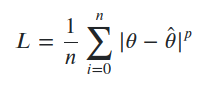
Loss (L) is a measurement of how well our model perform against your training data. You calculate loss using a loss function, many of which uses error in its equation; for example, simple loss functions may include:
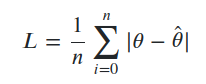
• Mean Absolute Error (MAE) – average of the errors

• Mean Squared Error (MSE) – average of the squares of the errors

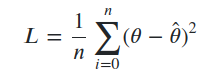
• Lp – MAE and MSE apply a power of 1 and 2 to the errors, respectively, and averages them. Because of this, they are also called L1 and L2 loss functions. However, you can apply higher (or negative) powers, or p, to the errors.

Whilst error is simply difference between θ and θ^, loss can differ depending on which loss function you pick. The loss function you pick depends on your data and your objectives. For instance, MAE, or L1, are sensitive to outliers; so if you want your model to also be sensitive to outliers, then you can use MAE.
Your loss depends on the loss function used, which depends on your use case; on the other hand, the error is always the same.
Risk
To re-iterate, loss measures how well your model fits against your training data. However, our end goal is not to fit our model to our training data, which can lead to overfitting. Instead, it is to fit against our validation and test data, or simply any new unseen data.
This is where (true) risk comes in. Risk is the average measure of loss, or expected loss, across your whole data distribution.
R(θ,θ^)=E[L(θ,θ^)]
To illustrate, let’s imagine that you have an overfitted model. Both the errors and loss of your model would be very low (because they are measured against your training data). But because it is overfitted, you’d expect the loss for any new data to be high. Thus, you have a model which has low error and loss, but very high risk.
Empirical Risk
To bring this back full circle – when we train our model, we do not have the full distribution of the data. This may be because some of our data is used for validation and testing, or that new data points are produced in real-time. The best we can do is to pick our training data in a random way and assume that our training data is representative of the real data.
Therefore, because we don’t have all the data, the best we can do is to minimize the empirical risk, from data that we do have (our training data), and use regularization techniques to generalize (i.e. avoid overfitting). This is why minimizing loss and minimizing empirical risk are roughly the same thing.

3) Occam’s razor states that when the simple explanation and complex explanation both work equally well, the simple explanation is usually correct. How do we apply this principle in ML?

https://machinelearningmastery.com/ensemble-learning-and-occams-razor/

In machine learning, Occam’s razor can be applied by favoring simpler models over complex ones if both achieve similar performance. This is because simpler models are generally easier to interpret and less prone to overfitting. Overfitting occurs when a model is too complex and performs well on the training data but poorly on new, unseen data. In contrast, simpler models are more likely to generalize well to new data, making them more useful in practice.
Therefore, when designing a machine learning system, it is important to strike a balance between model complexity and performance. This involves selecting a model architecture that is simple enough to avoid overfitting, but also powerful enough to capture the underlying patterns in the data. Additionally, techniques such as regularization and feature selection can be used to further simplify the model and reduce the risk of overfitting. Overall, the goal is to achieve the best possible performance with the simplest possible model.

4) What are the conditions that allowed deep learning to gain popularity in the last decade?

1. Availability of large amounts of labeled data: Deep learning models require large amounts of labeled data for training, which was made available due to the growth of the internet and advances in data storage and retrieval.
2. Increase in computational power: The development of graphical processing units (GPUs) made it possible to train deep neural networks in a reasonable amount of time.
3. Advances in algorithms: The development of new optimization algorithms, such as stochastic gradient descent, and regularization techniques, such as dropout, allowed for more efficient training of deep neural networks.
4. Open-source software: The availability of open-source software libraries, such as TensorFlow and PyTorch, made it easier for researchers and developers to build and experiment with deep learning models.
5. Industry investment: Major technology companies, such as Google, Microsoft, and Facebook, invested heavily in deep learning research and development, leading to breakthroughs in areas such as image and speech recognition.

5) If we have a wide NN and a deep NN with the same number of parameters, which one is more expressive and why?

A deep neural network (DNN) with the same number of parameters as a wide neural network (WNN) is generally more expressive. The reason for this is that DNNs are able to learn hierarchical representations of data, which can capture more complex and abstract relationships between features.
In a WNN, all the neurons in a layer are connected to all the neurons in the previous layer, resulting in a large number of connections. While this approach can work well for simple problems, it may not be as effective for more complex problems where there are many features and interactions between them.
In contrast, a DNN is composed of multiple layers, with each layer learning increasingly complex features based on the lower-level features learned in the previous layer. This allows the network to capture hierarchical representations of data, which can result in more expressive and powerful models.
Furthermore, a DNN can learn more compact representations of the input data, which can result in better generalization performance and improved ability to handle large and high-dimensional data.

6) The Universal Approximation Theorem states that a neural network with 1 hidden layer can approximate any continuous function for inputs within a specific range. Then why can’t a simple neural network reach an arbitrarily small positive error?

The Universal Approximation Theorem states that a neural network with one hidden layer can approximate any continuous function on a closed and bounded subset of Euclidean space. However, it does not specify the number of neurons or the size of the hidden layer required to achieve this approximation. In practice, a neural network with a single hidden layer may require an enormous number of neurons to achieve a good approximation for a given function, which can make training such a network computationally expensive and slow. Additionally, the theorem does not guarantee that the approximation error can be made arbitrarily small, which means that there may be some functions that cannot be approximated by a neural network with any finite number of parameters. Therefore, while the Universal Approximation Theorem provides a powerful theoretical foundation for neural networks, it does not necessarily imply that a simple neural network can achieve an arbitrarily small positive error.

7) What are saddle points and local minima? Which are thought to cause more problems for training large NNs?

Saddle points and local minima are critical points in the loss function of a neural network during training. A critical point is a point where the gradient of the loss function is zero, and it can be a minimum, maximum, or saddle point.
A local minimum is a critical point where the loss function has the smallest value in a small neighborhood but not necessarily the smallest value in the entire function. In other words, the loss function can be stuck in a local minimum, and it cannot decrease further, even if there exists a lower global minimum.
A saddle point is a critical point where the loss function has a flat region in one direction and a slope in another direction. It is called a saddle point because it resembles the shape of a saddle. At a saddle point, some dimensions have a positive gradient while others have a negative gradient, and the overall gradient of the loss function is close to zero. This can cause a slowdown in training since the weights are updated proportionally to the gradient, and small gradients lead to slow updates.
Both local minima and saddle points can cause problems for training large neural networks. While saddle points are more likely to be encountered in high-dimensional spaces, they may still slow down the optimization process by acting as a bottleneck. However, local minima can be more problematic since they can trap the optimization process and prevent the network from finding the global minimum of the loss function.

A saddle point is a critical point where the gradient of a function is zero but the Hessian matrix has both positive and negative eigenvalues. In other words, at a saddle point, the function is neither increasing nor decreasing in all directions, which can cause the gradient descent algorithm to slow down or converge to a suboptimal solution.
A local minimum is a critical point where the function has a lower value than all nearby points but may not be the global minimum of the function. A neural network can converge to a local minimum if the optimization algorithm gets stuck in a region where the gradient is close to zero, leading to suboptimal performance.
In general, saddle points are believed to cause more problems for training large neural networks than local minima. This is because saddle points are more common in high-dimensional spaces, and they can cause the optimization algorithm to get stuck for long periods. However, recent research has shown that the landscape of high-dimensional optimization problems is more complicated than just saddle points and local minima, and that other factors such as plateaus and valleys can also affect the performance of optimization algorithms.
https://www.khanacademy.org/math/multivariable-calculus/applications-of-multivariable-derivatives/optimizing-multivariable-functions/a/maximums-minimums-and-saddle-points

8) What are the differences between parameters and hyperparameters? Why is hyperparameter tuning important? Explain the algorithm for tuning hyperparameters.

1. Parameters are variables that are learned by the machine learning model during the training process. They are the internal variables that are used by the model to make predictions. In contrast, hyperparameters are the settings of the machine learning algorithm that cannot be learned from the data. They are set by the user before the training process and control the behavior of the learning algorithm, such as the learning rate, regularization strength, number of hidden layers, etc.
2. Hyperparameter tuning is important because the performance of a machine learning model heavily depends on the choice of hyperparameters. Choosing the right hyperparameters can lead to a model with high accuracy and generalization, while choosing the wrong hyperparameters can lead to overfitting or poor performance. Therefore, hyperparameter tuning is crucial to maximize the performance of a machine learning model.
3. The algorithm for tuning hyperparameters typically involves the following steps:

• Define a search space: specify the range or values of hyperparameters that will be considered during the search.
• Choose a search method: there are various methods for searching the hyperparameter space, such as grid search, random search, Bayesian optimization, etc.
• Define a performance metric: choose a metric to evaluate the performance of the model, such as accuracy, F1 score, or mean squared error.
• Train and evaluate the model: train the model using a combination of hyperparameters and evaluate its performance using the chosen metric.
• Iterate the search: repeat the previous step with different combinations of hyperparameters until the optimal combination is found.

The process of hyperparameter tuning can be time-consuming and computationally expensive, especially for large datasets and complex models. Therefore, it is important to choose a search method that balances the exploration of the hyperparameter space and the computational resources available.

Bayesian optimization is a technique used to find the best set of hyperparameters for a machine learning model. Hyperparameters are the settings that control the learning process of the algorithm, such as the learning rate, regularization strength, number of hidden layers, and number of neurons in each layer.
The idea behind Bayesian optimization is to construct a probability model that predicts the performance of the algorithm with a given set of hyperparameters. The model is updated with new evaluations of the algorithm’s performance as each set of hyperparameters is tried.
Bayesian optimization works by balancing exploration and exploitation. It explores new areas of the hyperparameter space by sampling from the model, and exploits areas where good performance has already been observed by focusing on the most promising regions.
The process starts with an initial set of hyperparameters, and then iteratively evaluates the performance of the algorithm with different hyperparameters. Based on the results, the probability model is updated, and the next set of hyperparameters to try is selected based on the model’s predictions.
This process continues until the best set of hyperparameters is found, or until a stopping criterion is met. Bayesian optimization is a powerful and efficient method for finding good hyperparameters, and is widely used in machine learning research and applications.
Bayesian optimization is a technique used to find the best set of hyperparameters for a machine learning model. Hyperparameters are the settings that control the learning process of the algorithm, such as the learning rate, regularization strength, number of hidden layers, and number of neurons in each layer.
The idea behind Bayesian optimization is to construct a probability model that predicts the performance of the algorithm with a given set of hyperparameters. The model is updated with new evaluations of the algorithm’s performance as each set of hyperparameters is tried.
Bayesian optimization works by balancing exploration and exploitation. It explores new areas of the hyperparameter space by sampling from the model, and exploits areas where good performance has already been observed by focusing on the most promising regions.
The process starts with an initial set of hyperparameters, and then iteratively evaluates the performance of the algorithm with different hyperparameters. Based on the results, the probability model is updated, and the next set of hyperparameters to try is selected based on the model’s predictions.
This process continues until the best set of hyperparameters is found, or until a stopping criterion is met. Bayesian optimization is a powerful and efficient method for finding good hyperparameters, and is widely used in machine learning research and applications.

Here’s an example of how Bayesian optimization might be used to tune hyperparameters for a machine learning model:
Suppose we have a dataset and a neural network architecture that we want to train on the data. We want to find the best set of hyperparameters (e.g. learning rate, regularization strength) for the neural network to maximize its performance on a validation set.
1. Define the search space: We first define a search space for the hyperparameters, such as a range of values or a set of discrete choices.
2. Choose an acquisition function: We then choose an acquisition function to guide the search process. This function measures the utility of evaluating the model with a certain set of hyperparameters and suggests which hyperparameters to try next. Examples of acquisition functions include expected improvement, upper confidence bound, and probability of improvement.
3. Choose an initial set of hyperparameters: We start with a set of hyperparameters chosen randomly or using some heuristics.
4. Evaluate the model with the chosen hyperparameters: We then evaluate the model’s performance with the chosen hyperparameters on the validation set.
5. Update the surrogate model: Based on the performance of the model, we update the surrogate model (e.g. Gaussian process regression) and calculate the acquisition function values for the remaining hyperparameters in the search space.
6. Choose the next set of hyperparameters: We then choose the next set of hyperparameters to evaluate based on the acquisition function.
7. Evaluate the model with the chosen hyperparameters and update the surrogate model again.
8. Repeat steps 5-7 until a stopping criterion is met (e.g. maximum number of iterations reached).
9. Choose the best set of hyperparameters: Finally, we choose the best set of hyperparameters based on the performance of the model on the validation set.
This process can be computationally expensive, but it can be very effective in finding the best set of hyperparameters for a machine learning model without requiring an exhaustive search.

9) What makes a classification problem different from a regression problem? Can a classification problem be turned into a regression problem and vice versa?

1. In a classification problem, the goal is to predict which category or class an observation belongs to, while in a regression problem, the goal is to predict a continuous numerical value. In other words, classification is about predicting a categorical outcome, while regression is about predicting a numerical outcome.
2. In some cases, it may be possible to turn a classification problem into a regression problem and vice versa, depending on the nature of the data and the problem at hand. For example, one could potentially turn a classification problem of predicting whether a person has a certain disease or not into a regression problem of predicting the probability of the person having the disease. Conversely, one could potentially turn a regression problem of predicting housing prices into a classification problem of predicting whether a house is affordable or not based on a certain threshold value. However, it is important to carefully consider the nature of the problem and the data before attempting to transform it into a different type of problem.

10) What’s the difference between parametric methods and non-parametric methods? Give an example of each method. When should we use one and when should we use the other?

Parametric algorithms
Parametric algorithms are based on a mathematical model that defines the relationship between inputs and outputs. This makes them more restrictive than nonparametric algorithms, but it also makes them faster and easier to train. Parametric algorithms are most appropriate for problems where the input data is well-defined and predictable.
Some examples of parametric algorithms include:
Linear regression — Linear regression is used to predict the value of a target variable based on a set of input variables. It is often used for predictive modeling tasks, such as predicting the sales volume of a product based on historical sales data.
Logistic regression — Logistic regression is used to predict the value of a target variable based on a set of input variables. It is often used for predictive modeling tasks, such as predicting the likelihood that a customer will purchase a product.
Neural network — Neural networks are a type of machine learning algorithm that are used to model complex patterns in data. Neural networks are inspired by the workings of the human brain, and they can be used to solve a wide variety of problems, including regression and classification tasks.
Nonparametric algorithms
Nonparametric algorithms are not based on a mathematical model; instead, they learn from the data itself. This makes them more flexible than parametric algorithms but also more computationally expensive. Nonparametric algorithms are most appropriate for problems where the input data is not well-defined or is too complex to be modelled using a parametric algorithm.
Some examples of nonparametric algorithms include:
Decision trees — Decision trees are a type of nonparametric machine learning algorithm that are used to model complex patterns in data. Decision trees are based on a hierarchical structure, and they can be used to solve a wide variety of problems, including regression and classification tasks.
Support vector machine — A support vector machine is a type of machine learning algorithm that is used for data classification tasks. SVMs are particularly well-suited for tasks where the input data is linearly separable. This means that the data can be separated into distinct classes or groups using a linear boundary.
When to use a parametric algorithm?
Parametric algorithms are best suited for problems where the input data is well-defined and predictable. This makes them ideal for tasks such as predictive modelling, where the goal is to predict the value of a target variable based on a set of input variables.
Example: Let’s say you want to predict the sales volume of a product. You would use a parametric algorithm, such as linear regression, to build a model that defines the relationship between historical sales data and the predicted sales volume.
When to use a nonparametric algorithm?
Nonparametric algorithms are best suited for problems where the input data is not well-defined or too complex to be modelled using a parametric algorithm. This makes them ideal for tasks such as data classification, where the goal is to separate data into distinct classes or groups. Additionally, nonparametric algorithms are often more accurate than parametric algorithms for complex problems.
Example: Let’s say you want to build a machine learning algorithm to predict the price of a stock based on historical data. In this case, you would use a parametric algorithm, such as linear regression. This is because the input data (historical stock prices) is well-defined and predictable. On the other hand, if you want to build an algorithm to classify images of animals, you would use a nonparametric algorithm, such as a support vector machine. This is because the input data (images of animals) is not well-defined and too complex to be modelled using a parametric algorithm.

Parametric Machine Learning Algorithms
Assumptions can greatly simplify the learning process, but can also limit what can be learned. Algorithms that simplify the function to a known form are called parametric machine learning algorithms.
A learning model that summarizes data with a set of parameters of fixed size (independent of the number of training examples) is called a parametric model. No matter how much data you throw at a parametric model, it won’t change its mind about how many parameters it needs.
— Artificial Intelligence: A Modern Approach, page 737
The algorithms involve two steps:
1. Select a form for the function.
2. Learn the coefficients for the function from the training data.
An easy to understand functional form for the mapping function is a line, as is used in linear regression:
b0 + b1x1 + b2x2 = 0
Where b0, b1 and b2 are the coefficients of the line that control the intercept and slope, and x1 and x2 are two input variables.
Assuming the functional form of a line greatly simplifies the learning process. Now, all we need to do is estimate the coefficients of the line equation and we have a predictive model for the problem.
Often the assumed functional form is a linear combination of the input variables and as such parametric machine learning algorithms are often also called “linear machine learning algorithms“.
The problem is, the actual unknown underlying function may not be a linear function like a line. It could be almost a line and require some minor transformation of the input data to work right. Or it could be nothing like a line in which case the assumption is wrong and the approach will produce poor results.
Some more examples of parametric machine learning algorithms include:
• Logistic Regression
• Linear Discriminant Analysis
• Perceptron
• Naive Bayes
• Simple Neural Networks
Benefits of Parametric Machine Learning Algorithms:
• Simpler: These methods are easier to understand and interpret results.
• Speed: Parametric models are very fast to learn from data.
• Less Data: They do not require as much training data and can work well even if the fit to the data is not perfect.
Limitations of Parametric Machine Learning Algorithms:
• Constrained: By choosing a functional form these methods are highly constrained to the specified form.
• Limited Complexity: The methods are more suited to simpler problems.
• Poor Fit: In practice the methods are unlikely to match the underlying mapping function.

Nonparametric Machine Learning Algorithms
Algorithms that do not make strong assumptions about the form of the mapping function are called nonparametric machine learning algorithms. By not making assumptions, they are free to learn any functional form from the training data.
Nonparametric methods are good when you have a lot of data and no prior knowledge, and when you don’t want to worry too much about choosing just the right features.
— Artificial Intelligence: A Modern Approach, page 757
Nonparametric methods seek to best fit the training data in constructing the mapping function, whilst maintaining some ability to generalize to unseen data. As such, they are able to fit a large number of functional forms.
An easy to understand nonparametric model is the k-nearest neighbors algorithm that makes predictions based on the k most similar training patterns for a new data instance. The method does not assume anything about the form of the mapping function other than patterns that are close are likely to have a similar output variable.
Some more examples of popular nonparametric machine learning algorithms are:
• k-Nearest Neighbors
• Decision Trees like CART and C4.5
• Support Vector Machines
Benefits of Nonparametric Machine Learning Algorithms:
• Flexibility: Capable of fitting a large number of functional forms.
• Power: No assumptions (or weak assumptions) about the underlying function.
• Performance: Can result in higher performance models for prediction.
Limitations of Nonparametric Machine Learning Algorithms:
• More data: Require a lot more training data to estimate the mapping function.
• Slower: A lot slower to train as they often have far more parameters to train.
• Overfitting: More of a risk to overfit the training data and it is harder to explain why specific predictions are made.

https://vitalflux.com/difference-between-parametric-vs-non-parametric-models/
https://machinelearningmastery.com/parametric-and-nonparametric-machine-learning-algorithms/

11) Why does ensembling independently trained models generally improve performance?

Ensembling independently trained models generally improves performance because it combines the strengths of multiple models and reduces the impact of individual weaknesses.
Each machine learning model has its own biases and limitations, and no single model can accurately capture all the complexities of a given dataset. By training multiple models independently and then combining their predictions, ensembling can help mitigate these biases and limitations and produce a more accurate and robust prediction.
There are different types of ensembling techniques, including bagging, boosting, and stacking. Bagging, or bootstrap aggregating, involves training multiple models on different subsets of the training data and then aggregating their predictions. This can reduce overfitting and improve accuracy. Boosting, on the other hand, involves training multiple models sequentially, where each model learns from the errors of the previous model. This can improve the model’s performance on hard-to-predict cases. Stacking involves training multiple models and then using their predictions as inputs to a meta-model that learns to combine them.
Overall, ensembling independently trained models is a powerful technique for improving the performance of machine learning models. It can lead to better accuracy, more robust predictions, and improved generalization to new data.

12) Why does L1 regularization tend to lead to sparsity while L2 regularization pushes weights closer to 0?

Distance is calculated between points and Norm calculated between vectors
What is Norm?
In simple words, the norm is a quantity that describes the size of a vector, something that we can represent using a set of numbers as you might already know that in machine learning everything is represented in terms of vectors. In this norm, all the components of the vector are weighted equally.
let’s take vector ‘a’ that contains two elements X1 and X2. We can represent the features of vector ‘a’ in two-dimensional (2d).
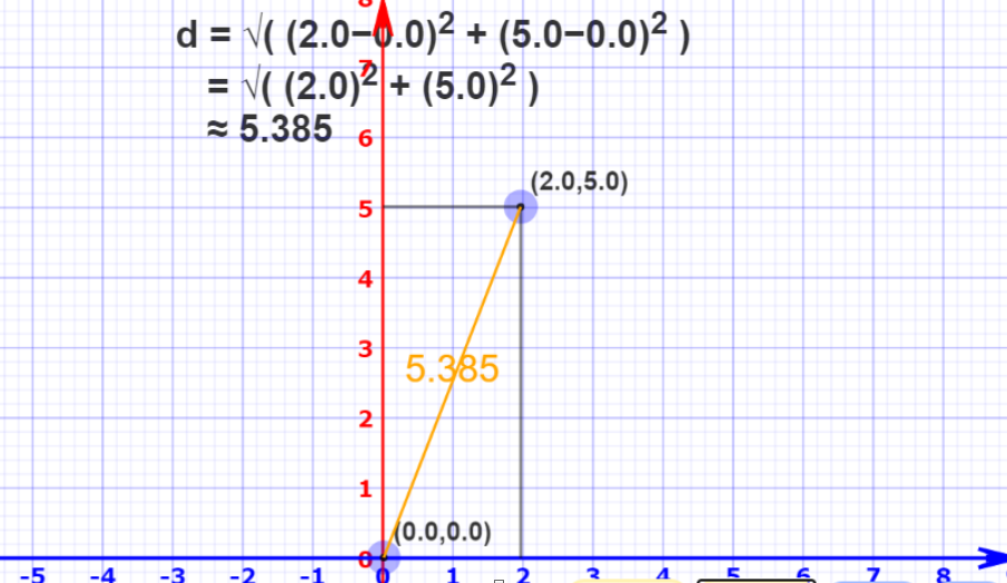
a = (2,5) and O(0,0)
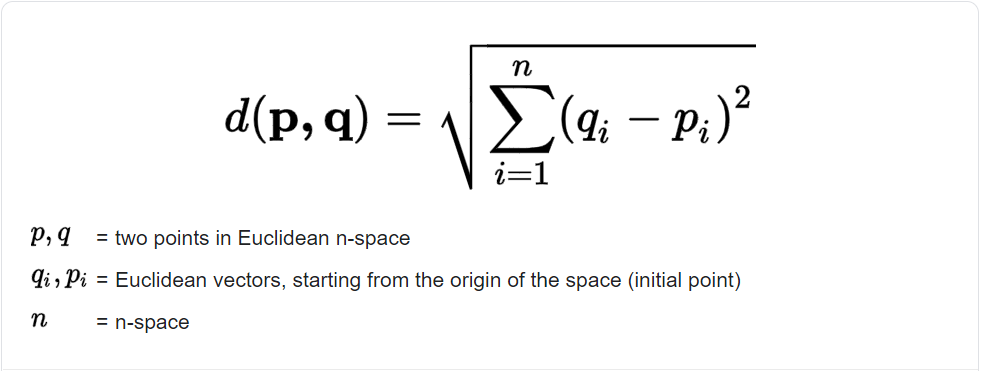
1. L2 Norm / Euclidean distance
Let’s calculate the distance of point a from the origin (0,0) using the l2 norm, which is also known as Euclidean distance.

L1 Norm / Manhattan distance
We can also calculate distance using another way to measure the size of the vector by effectively adding all the components of the vector and this is called the Manhattan distance a.k.a L1 norm.
Manhattan distance = ||X1-X2||1 ~ (summation(abs(X1i-X2i)))
Manhattan Distance [{a, b}, {x, y}] = Abs [a − x] + Abs [b − y]
[{0,0} , {2,5}] = |0–2| + |0–5| = |-2|+|-5| = 2+5 = 7
The generalize equation of ln norm is the nth root of the summation of all components to their nth powers.

L-infinity norm

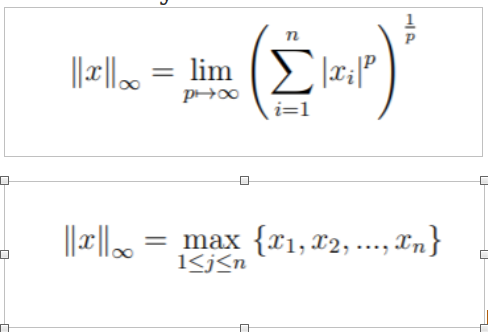
Gives the largest magnitude among each element of a vector.
Having the vector X= [-6, 4, 2], the L-infinity norm is 6.
In the L-infinity norm, only the largest element has any effect. So, for example, if your vector represents the cost of constructing a building, by minimizing the L-infinity norm we are reducing the cost of the most expensive building.

The behavior of the norms

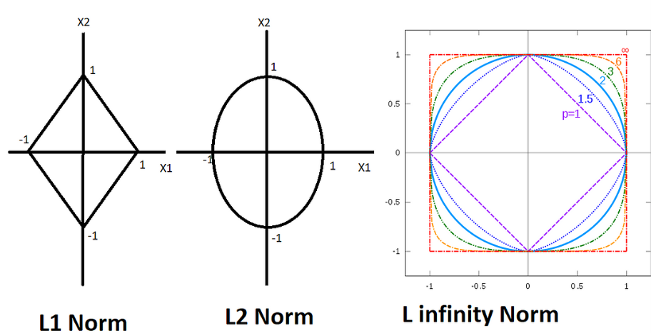
The plot describes the behavior of every vector that has an L1 norm equal to 1. Every point on the circumference of the square is a vector with L1 norm = 1 but what happens when we do it for the l2 norm? It becomes a circle and it’s actually easy to guess because in the equation of the circle in 2d there are square terms right and in the formula of l2 norm there are squares
so it makes sense right every point on the circumference of the circle has l2 norm as one let’s see what happens to the circle as we increase n.
we can clearly see that as we increase the order the shape approaches a square but wait how did I even calculate the L infinity norm well I just took the limit of the formula as n approaches infinity it turns out that L infinity is just the maximum component of the vector now that we have a very good
understanding of the norms.
Where norms are used the most common?
1. Mean Squared Error
2. Ridge Regression Constraint
3. Lasso Regression Constraint
Mean Squared Error: The mean squared error (MSE) or mean squared deviation (MSD) of an estimator (of a procedure for estimating an unobserved quantity) measures the average of the squares of the errors — that is, the average squared difference between the estimated values and the actual value.

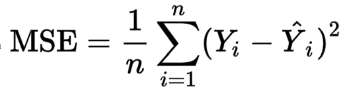
n = number of data points ; Y_{i} = observed values ; Y(hat)_{i} = predicted values
The error cost function is the sum of the squared differences between ground truths and predictions are nothing but the l2 norm of the resultant vector formed by subtracting the vector of predictions from the vector of ground truths.

Ridge Regression Constraint :
we put a constraint on the weights and the constraint says nothing but the l to the norm of the weight vector should be greater than or equal to some positive value visually the optimized weight vector should lie outside the red circle.

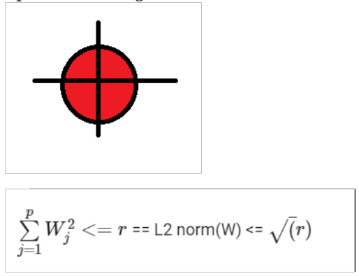
L2 norm equation.
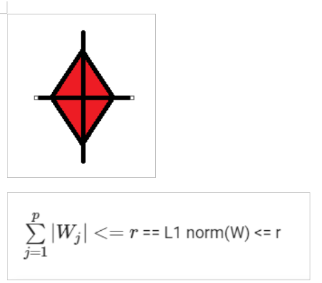
Lasso Regression Constraint :
If we talk about lasso regression then the constraint becomes l1 norm and in this case, the optimized weight vector should lie outside the red square.

Why L1 norm creates Sparsity?
We gonna have a quick tour on why the l1 norm is so useful for promoting sparse solutions to linear systems of equations. The reason for using the L1 norm to find a sparse solution is due to its special shape. It has spikes that happen to be at sparse points. Using it to touch the solution surface will very likely to find a touch point on a spike tip and thus a sparse solution.

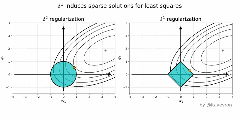
The above figure is the geometric perspective on sparsity and the L1 norm and L2 norm.

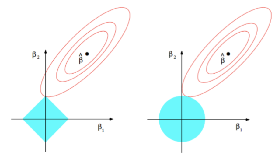
The solid blue areas are the constraint regions |β1|+|β2| ≤ r and β1² + β2² ≤ t², respectively, while the res ellipses are the contours of the least squared error functions.
The β^ is the unconstrained least squares estimate. The red ellipses are (as explained in the caption of this Figure) the contours of the least-squares error function, in terms of parameters β1 and β2. Without constraints, the error function is minimized at the MLE β^, and its value increases as the red ellipses out expand. The diamond and disk regions are feasible regions for lasso (L1) regression and ridge (L2) regression respectively. Heuristically, for each method, we are looking for the intersection of the red ellipses and the blue region as the objective is to minimize the error function while maintaining feasibility.
That being said, it is clear to see that the L1 constraint, which corresponds to the diamond feasible region, is more likely to produce an intersection that has one component of the solution is zero (i.e., the sparse model) due to the geometric properties of ellipses, disks, and diamonds. It is simply because diamonds have corners (of which one component is zero) that are easier to intersect with the ellipses that extending diagonally.

13) Why does an ML model’s performance degrade in production?

Machine learning models can experience degradation in performance when they are deployed in production for several reasons, including:
1. Data Drift: The model may have been trained on a specific dataset, but the real-world data that it encounters in production may be different. This can result in a phenomenon known as data drift, where the statistical properties of the data change over time, causing the model’s predictions to become less accurate. The model may need to be retrained or updated to adapt to the new data.
2. Concept Drift: Concept drift occurs when the underlying relationship between the input variables and the output variable changes over time. This can happen, for example, if the behavior of the users or the environment changes in a way that was not captured in the training data. The model may need to be re-evaluated and updated to handle these changes.
3. Overfitting: In some cases, a model may have been overfit to the training data, meaning that it has learned to fit the noise or random variations in the data rather than the underlying patterns. This can cause the model’s performance to degrade when it encounters new data. Regularization techniques can be used during training to help prevent overfitting.
4. Scaling: The performance of a model may change when it is deployed to a larger scale than the training environment. Issues like hardware limitations, network bandwidth, and software inefficiencies can all impact the performance of a model in production. Proper testing and benchmarking can help to identify these issues.
5. Maintenance: Lastly, a model may degrade in performance due to maintenance issues, such as outdated dependencies, incorrect configuration, or poor monitoring. Regular maintenance and monitoring can help to prevent these issues from affecting the model’s performance.
Overall, it is important to carefully monitor a machine learning model in production and regularly evaluate its performance to ensure that it continues to perform well over time.

14) What problems might we run into when deploying large machine learning models?

Deploying large machine learning models can present several challenges and problems, including:
1. Memory and Storage Requirements: Large machine learning models can require a significant amount of memory and storage, which can make them challenging to deploy on resource-constrained systems. This can result in longer load times, increased latency, and higher infrastructure costs.
2. Computation Requirements: Large machine learning models can also be computationally expensive to evaluate, which can cause performance issues in production. This can result in longer response times, increased latency, and higher infrastructure costs.
3. Network Bandwidth: Transmitting large machine learning models over a network can be challenging, particularly in situations where network bandwidth is limited or unreliable. This can impact the speed and accuracy of predictions.
4. Deployment Environment: Deploying large machine learning models can also be challenging due to the complexity of the deployment environment. Issues like system compatibility, version conflicts, and software dependencies can all impact the deployment process and introduce potential errors.
5. Security: Large machine learning models can contain sensitive information, such as personally identifiable information (PII) or intellectual property (IP), which can make them vulnerable to cyber attacks. Proper security measures, such as data encryption and access control, must be implemented to protect against these threats.
6. Explainability: Large machine learning models can also be challenging to interpret and explain, particularly when they involve complex architectures like deep neural networks. This can make it difficult to understand how the model arrived at a particular prediction or decision.
Overall, deploying large machine learning models requires careful consideration and planning to ensure that they can be effectively deployed in a production environment while maintaining performance, security, and interpretability

https://neptune.ai/blog/model-deployment-challenges-lessons-from-ml-engineers

https://censius.ai/blogs/challenges-in-deploying-machine-learning-models

15) Your model performs really well on the test set but poorly in production. What are your hypotheses about the causes? How do you validate whether your hypotheses are correct? Imagine your hypotheses about the causes are correct. What would you do to address them?

There could be several reasons why a model performs well on the test set but poorly in production, some possible hypotheses are:
1. Data distribution shift: The test set and production data have different underlying distributions, causing the model to perform poorly on production data.
2. Data quality issues: The production data may contain outliers, missing values, or other data quality issues that were not present in the test set, leading to poor model performance.
3. Model overfitting: The model may have overfit the training data and performed well on the test set due to chance, but fails to generalize to production data.
4. Model complexity: The model may be too complex for the production environment, leading to poor performance in production.
5. Model architecture or hyperparameters: The model architecture or hyperparameters may be optimized for the test set but not for the production environment, leading to poor performance in production.
6. Deployment issues: The model may not have been deployed correctly in the production environment, leading to poor performance.

To validate the hypotheses, we can perform several steps. First, we can evaluate the model’s performance on a validation set that is representative of the production environment. If the model performs poorly on the validation set, it indicates that the model is not generalizing well to the production environment. Second, we can analyze the data distribution and quality in the production environment and compare it to the training and test sets. If there are significant differences, we may need to retrain the model with more representative data or perform additional feature engineering. Third, we can perform A/B testing to compare the performance of the new model with the old model in the production environment and validate the hypothesis.

1. Conduct data analysis: Analyze the production data and compare it to the test set to identify any differences in data distribution or quality.
2. Conduct model analysis: Analyze the model’s performance on the production data and compare it to the test set to identify any differences in performance.
3. Conduct experiments: Conduct experiments to test the impact of changes in data or model on performance in production.
4. Conduct A/B testing: Deploy multiple versions of the model in production and compare their performance to identify the cause of poor performance.
5. Conduct root cause analysis: Analyze the system and infrastructure where the model is deployed to identify any issues that may be causing poor performance.
6. Gather feedback: Gather feedback from users and stakeholders to understand their experience and identify any issues that may be impacting performance.

These steps can help validate the hypotheses about the causes of poor model performance in production and identify the necessary actions to improve performance.

If the hypotheses are correct, we can take several steps to address them. If overfitting is the problem, we may need to use techniques such as regularization or early stopping to prevent the model from overfitting to the test set. If there are differences in the data distribution or quality, we may need to collect more representative data or perform additional feature engineering to better capture the characteristics of the production environment. We may also need to validate the model’s output in the production environment using techniques such as A/B testing or monitoring the model’s performance over time to detect and correct any errors in the model deployment process.

If the hypotheses about the causes of poor model performance in production are correct, there are several possible actions that can be taken to address them:
1. Re-evaluate the training process: If the issue is related to the training data, re-evaluating the data selection and preprocessing methods, or collecting new data that is more representative of the production data, may help improve the model’s performance.
2. Improve feature engineering: If the issue is related to the features used for training the model, improving the feature engineering process or introducing new features may improve the model’s performance.
3. Re-train the model: If the issue is related to the model architecture or hyperparameters, re-training the model with different settings or architectures may help improve its performance.
4. Regular model maintenance: Implement regular model maintenance to ensure the model remains up to date with changes in production data and remains robust to new scenarios.
5. Redesign the production infrastructure: If the issue is related to the infrastructure or deployment environment, redesigning the infrastructure, or making changes to the deployment process may help improve the model’s performance in production.
6. Conduct ongoing monitoring and analysis: Set up monitoring processes to continuously monitor the model’s performance in production and analyze the data to identify any potential issues or trends that may affect the model’s performance.
By addressing the underlying causes of poor model performance in production, these actions can help improve the model’s performance and ensure it meets the required levels of accuracy and reliability.