Machine Learning Interview: Training Neural Networks
2021-07-02Best practices for Python exceptions
2021-07-251) For neural networks that work with images like VGG-19, InceptionNet, you often see a visualization of what type of features each filter captures. How are these visualizations created?
Hint: check out this Distill post on Feature Visualization.
The visualizations of filters in deep neural networks are created through a process called “feature visualization” or “activation maximization”.
In essence, the goal is to find an input image that maximizes the activation of a particular filter or neuron in the network. By optimizing the input image to excite a certain filter, we can visualize the type of features that the filter is detecting.
Here are the basic steps to create these visualizations:
- Choose a layer in the neural network that contains filters you want to visualize.
- Select a specific filter from that layer.
- Generate a random noise image or an initial image to start with.
- Forward propagate this initial image through the network up to the chosen layer, and compute the activation of the selected filter.
- Backpropagate the gradients from the activation of the selected filter to the input image pixels, and adjust the pixel values to increase the activation of the filter.
- Repeat steps 4 and 5 iteratively, each time adjusting the input image to increase the activation of the selected filter.
- Continue the optimization until the filter is maximally activated, and then visualize the optimized image as the pattern or feature that the filter is detecting.
There are variations and enhancements to this basic process, such as using different regularization techniques to avoid overfitting or smoothing the resulting image for better visual quality, but the basic principle is the same: iteratively adjust the input image to increase the activation of the desired filter and visualize the resulting image.
2) How are your model’s accuracy and computational efficiency affected when you decrease or increase its filter size? How do you choose the ideal filter size?
Example: Kernel with size 1×1 give the next layer the same number of neuron; kernel with size NxN give only one neuron in the next layer.
The impact of a larger kernel:
- Computational time is faster, memory usage is smaller
- Loss a lot of details. Imagine NxN input neuron and the kernel size is NxN too, then the next layer only gives you one neuron. Loss a lot of details can lead you to underfitting.
A smaller kernel will give you a lot of details, which can lead you to overfitting, but a larger kernel will give you loss a lot of details, it can lead you to underfitting. You should tune your model to find the best size. Sometimes, time and machine specifications should be considered
In Convolutional Neural Networks (CNNs), the filter size determines the receptive field of each convolutional layer. The receptive field is the region of the input image that the neuron in the current layer is connected to.
When you decrease the filter size in CNNs:
- Accuracy: Smaller filters can capture finer-grained details and patterns in the input image. This can increase the network’s accuracy, especially in tasks that require fine-grained classification, such as object detection or image segmentation. However, if the filters are too small, they may miss out on larger patterns and structures in the image, leading to lower accuracy.
- Computational efficiency: Smaller filters require fewer parameters to train, which can reduce the computational complexity and memory requirements of the network. Smaller filters can also result in faster training and inference times, as there are fewer computations to perform per layer.
When you increase the filter size in CNNs:
- Accuracy: Larger filters can capture more global patterns and structures in the input image. This can improve the network’s accuracy, especially in tasks that require understanding of global context, such as scene recognition or image classification. However, if the filters are too large, they may also capture noise or irrelevant information, leading to lower accuracy.
- Computational efficiency: Larger filters require more parameters to train, which can increase the computational complexity and memory requirements of the network. Larger filters can also result in slower training and inference times, as there are more computations to perform per layer.
In summary, the choice of filter size in CNNs depends on the specific task and dataset. For fine-grained tasks, smaller filters may be more effective, while for tasks that require global context, larger filters may be more effective. However, the choice of filter size is often a trade-off between accuracy and computational efficiency.
Choosing the ideal filter size for a convolutional neural network (CNN) depends on several factors, including the specific task, the dataset, and the network architecture. Here are some general guidelines to help you choose an appropriate filter size:
- Consider the size of the objects or patterns you want to detect: If the objects or patterns in your dataset are small, using smaller filter sizes may be more effective. Conversely, if the objects or patterns are large, using larger filter sizes may be more effective.
- Consider the spatial resolution of the input image: If your input images have high spatial resolution, using smaller filter sizes may be more effective since they can capture more fine-grained details. If your input images have low spatial resolution, using larger filter sizes may be more effective since they can capture more global patterns.
- Consider the depth of the network: In deeper networks, using smaller filter sizes can help capture more local patterns and details, while using larger filter sizes can help capture more global patterns. It is common to use a combination of both small and large filter sizes in deep networks.
- Experiment with different filter sizes: It is often useful to experiment with different filter sizes and observe their impact on the network’s performance. Try training the network with different filter sizes and compare their accuracy and computational efficiency.
- Use pre-trained models: If you are working with limited resources or limited training data, it may be beneficial to use pre-trained models with established filter sizes. This can save time and resources while still achieving high accuracy.
In general, the ideal filter size is highly dependent on the specific task and dataset, and may require some trial and error to determine. However, by considering the factors listed above, you can make an informed decision on an appropriate filter size for your CNN.
Choosing the ideal filter size in Convolutional Neural Networks (CNNs) is an important task, as it can have a significant impact on the performance of the network. Here are some factors to consider when choosing the filter size:
- Task: The filter size should be chosen based on the specific task that the CNN is being used for. For example, for object detection or image segmentation tasks that require fine-grained details, smaller filter sizes may be more effective, while for image classification tasks that require capturing global features, larger filter sizes may be more effective.
- Input image size: The filter size should also be chosen based on the size of the input image. If the input image is large, larger filters may be more effective in capturing global features, while if the input image is small, smaller filters may be more effective in capturing fine-grained details.
- Network architecture: The choice of filter size should also take into account the architecture of the CNN. For example, if the CNN has many layers, smaller filters may be more effective in capturing finer-grained details, while if the CNN has fewer layers, larger filters may be more effective in capturing global features.
- Computational resources: The choice of filter size should also consider the computational resources available. Larger filters require more parameters and computational resources, while smaller filters require fewer parameters and computational resources.
- Experimentation: Finally, it is important to experiment with different filter sizes and evaluate the performance of the CNN on the task at hand. This can help identify the optimal filter size that balances accuracy and computational efficiency.
In summary, choosing the ideal filter size in CNNs requires consideration of the task, input image size, network architecture, computational resources, and experimentation.
3) Convolutional layers are also known as “locally connected.” Explain what it means.
Convolutional layers in a Convolutional Neural Network (CNN) are often referred to as “locally connected” layers because they perform a convolution operation with a small kernel or filter, which is applied locally to each region of the input image.
In a locally connected layer, each neuron in the layer is only connected to a small region of the input image, known as the receptive field. This local connectivity is achieved through the use of convolutional filters that are applied to small patches of the input image. These filters are often much smaller than the input image itself, and they slide across the entire image, computing the dot product of the filter and the input patch at each location. This produces a feature map that highlights the presence of certain patterns or features in the input image.
By applying filters locally to each region of the input image, convolutional layers can capture local spatial dependencies and patterns, while also being invariant to translation. This is particularly useful in computer vision tasks such as object recognition, where the position of an object in the input image can vary.
In contrast to fully connected layers, where each neuron is connected to every neuron in the previous layer, locally connected layers reduce the number of parameters in the network by sharing weights across the input image. This reduces the memory requirements and computational complexity of the network, making it more efficient to train and use.
In summary, convolutional layers in a CNN are called “locally connected” because they perform a convolution operation with a small kernel or filter, which is applied locally to each region of the input image, enabling the network to capture local spatial dependencies and patterns while being invariant to translation.
Convolutional layers are technically locally connected layers. To be precise, they are locally connected layers with shared weights. We run the same filter for all the (x,y) positions in the image. In other words, all the pixel positions “share” the same filter weights. We allow the network to tune the filter weights until we arrive at the desired performance. While this is great at image classification tasks, we tend to miss out on some subtle nuances of spatial arrangements.
4) When we use CNNs for text data, what would the number of channels be for the first conv layer?
When we use Convolutional Neural Networks (CNNs) for text data, the number of channels for the first convolutional layer would depend on the representation of the text input.
If we are using a one-hot encoding representation of the text, each word in the input would be represented by a binary vector with a dimension equal to the size of the vocabulary. In this case, we would typically use a single channel for the first convolutional layer, where each filter would slide over the input sequence of one-hot vectors. The output feature maps would highlight the presence of certain patterns or n-grams in the input sequence.
Alternatively, if we are using a pre-trained word embedding representation of the text, each word in the input would be represented by a dense vector with a fixed dimension. In this case, we would typically use a multi-channel approach for the first convolutional layer, where each channel corresponds to a different embedding dimension. For example, if we are using a 100-dimensional word embedding, the first convolutional layer might have 100 channels, where each filter would slide over the input sequence of 100-dimensional word vectors. The output feature maps would capture different patterns or relationships between the embedding dimensions.
In summary, the number of channels for the first convolutional layer in CNNs for text data depends on the representation of the text input. For one-hot encoding, we typically use a single channel, while for pre-trained word embeddings, we typically use multiple channels corresponding to the embedding dimensions.
https://medium.com/voice-tech-podcast/text-classification-using-cnn-9ade8155dfb9
What is the role of zero padding?
Zero padding is a technique that allows us to preserve the original input size. This is something that we specify on a per-convolutional layer basis. With each convolutional layer, just as we define how many filters to have and the size of the filters, we can also specify whether or not to use padding.
What Is Zero Padding?
We now know what issues zero padding combats against, but what actually is it?
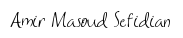
Zero padding occurs when we add a border of pixels all with value of zero around the edges of the input images. This adds kind of a padding of zeros around the outside of the image, hence the name zero padding. Going back to our small example from earlier, if we pad our input with a border of zero valued pixels, let’s see what the resulting output size will be after convolving our input.
We see that our output size is indeed 4 x 4, maintaining the original input size. Now, sometimes we may need to add more than a border that’s only a single pixel thick. Sometimes we may need to add something like a double border or triple border of zeros to maintain the original size of the input. This is just going to depend on the size of the input and the size of the filters.
Valid And Same Padding
There are two categories of padding. One is referred to by the name valid. This just means no padding. If we specify valid padding, that means our convolutional layer is not going to pad at all, and our input size won’t be maintained.
The other type of padding is called same. This means that we want to pad the original input before we convolve it so that the output size is the same size as the input size.
| Padding Type | Description | Impact |
| Valid | No padding | Dimensions reduce |
| Same | Zeros around the edges | Dimensions stay the same |
Zero padding is a technique used in Convolutional Neural Networks (CNNs) to increase the spatial size of the output feature maps from convolutional layers. It involves adding zeros to the input image around the border, effectively increasing its size before performing the convolution operation.
The main role of zero padding is to preserve the spatial resolution of the input image as it passes through the convolutional layers. Without zero padding, the size of the output feature maps would be reduced with each convolutional layer, as the filter “slides” across the image and only computes values for pixels that are fully covered by the filter. This reduction in spatial resolution can result in a loss of important information about the input image.
By adding zeros to the input image before the convolution operation, zero padding ensures that the output feature maps have the same spatial size as the input image. This is important for tasks such as object detection or image segmentation, where precise spatial information is required.
Another benefit of zero padding is that it can help reduce the impact of the boundary pixels on the output feature maps. Without zero padding, the boundary pixels of the input image are only processed by the filter once, resulting in lower weights for these pixels. With zero padding, the boundary pixels are processed multiple times, resulting in higher weights and better representation of the boundary regions in the output feature maps.
In summary, the role of zero padding in CNNs is to preserve the spatial resolution of the input image as it passes through the convolutional layers, and to improve the representation of the boundary regions.
5) Why do we need upsampling? How to do it?
In Convolutional Neural Networks (CNNs), upsampling is a technique used to increase the resolution of feature maps and improve the performance of the network. Here are some reasons why we need upsampling in CNNs:
- Recover lost spatial information: In CNNs, the resolution of feature maps decreases as we move deeper into the network. This is due to the pooling operations that are commonly used to downsample the feature maps. Upsampling can be used to recover the lost spatial information and increase the resolution of the feature maps.
- Generate high-resolution outputs: In tasks such as image segmentation, where we need to generate pixel-wise predictions, it is important to have high-resolution feature maps. Upsampling can be used to increase the resolution of the feature maps before generating the output.
- Improve performance: Upsampling can be used to improve the performance of the network by increasing the number of parameters and providing more detailed feature maps for downstream layers to work with. By increasing the number of parameters, we can increase the capacity of the network and learn more complex representations.
Suppose we want the output to be the same size as the input “Imagine you are in a semantic segmentation task where every pixel of the input will assigned to a label so you need an output of the same size of input”. Meaning we need to reverse the “Downsampling”.
Starting with a small size image, we need to reach the previous size. “actually we just need to reach to the same size not to the exact features map”, this is what is called Upsampling
And this is the second half of a fully convolution network that seeks to return to the original size.
There are many ways to do this.
Different ways for upsampling:
There are several ways to perform upsampling in CNNs, including transposed convolution, bilinear interpolation, and nearest-neighbor interpolation. Each method has its advantages and disadvantages, and the choice of upsampling method depends on the specific task and the architecture of the network.
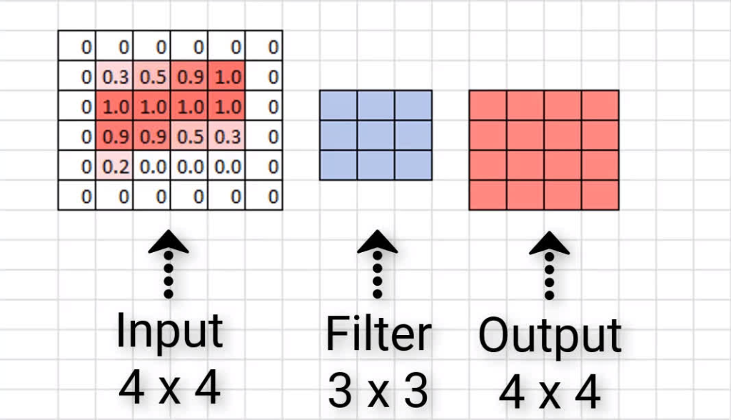
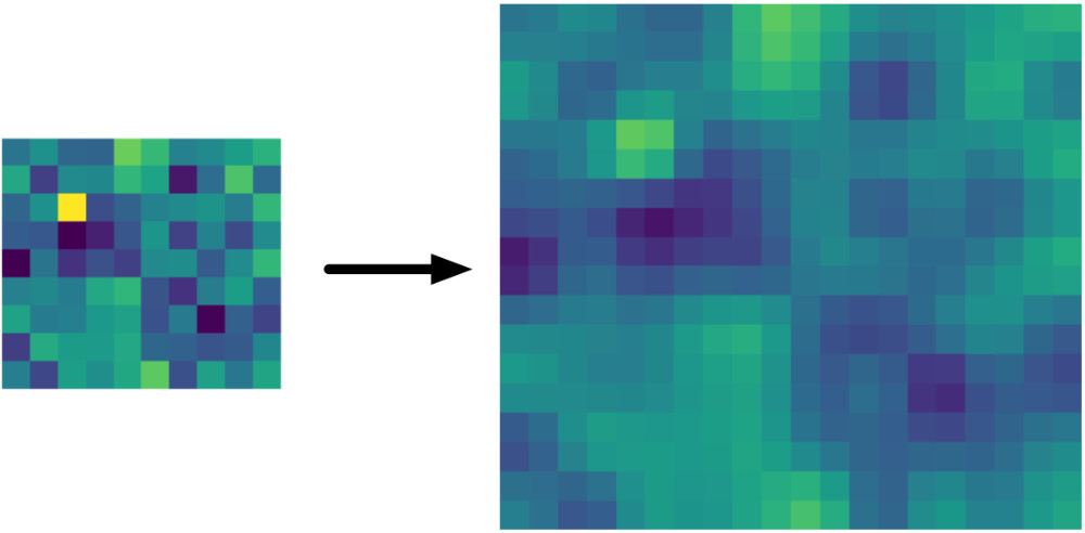
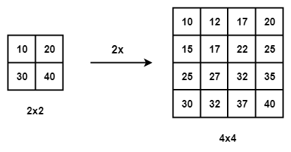
- Simple upsampling (Nearest neighbor) :
from its name it is a very simple and computationally cheap operation it just copies or repeats the rows and then the columns according to the upsampling factor.
Here the upsampling factor is (2,2) so doubling the rows and then doubling the columns leads to an increase in the output size.
With the easy implementation in Keras :
tf.keras.layers.UpSampling2D(
size=(2, 2), data_format=None, interpolation=”nearest”, **kwargs
)
where size is the upsampling factor and data_format is where the channel is first or last.
- Un-pooling :
Instead of naive repeating of pixels, we can just reverse the operation used in downsampling, reversing pooling with Un-pooling as follows:
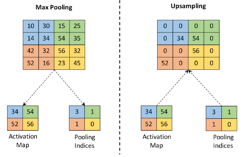
Not returning to the same exact pixels but at least to the same resolution with the most important pixels.
- Transpose convolution :
OR we can reverse the convolution layers using what is said Transpose convolution or deconvolution “which is a mathematically incorrect term” or unconv or partially stride convolution and it is the most common way for upsampling, we just transpose what happened in the regular convolution as following.
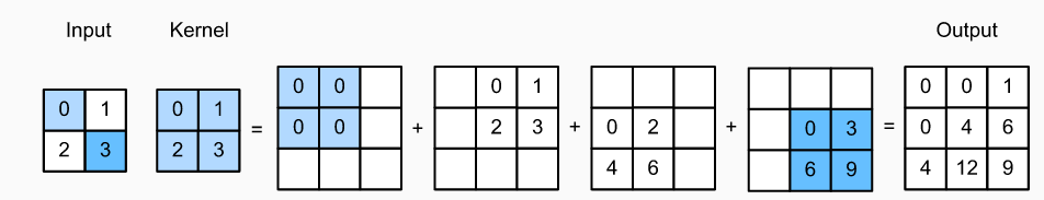
each pixel of the input is multiplied with the kernel and put the output(the same as the kernel size) in the final output feature map and moves again with a stride (but this time stride to the output), So here increasing the stride will increase the output size, on the other hand increasing the padding will decrease the output size.
Bi-Linear Interpolation: In Bi-Linear Interpolation, we take the 4 nearest pixel values of the input pixel and perform a weighted average based on the distance of the four nearest cells smoothing the output.
Bi-Linear Interpolation
Bed Of Nails: In Bed of Nails, we copy the value of the input pixel at the corresponding position in the output image and fill in zeros in the remaining positions.
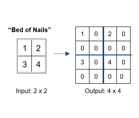
Bed Of Nails Upsampling
Max-Unpooling: The Max-Pooling layer in CNN takes the maximum among all the values in the kernel. To perform max-unpooling, first, the index of the maximum value is saved for every max-pooling layer during the encoding step. The saved index is then used during the Decoding step where the input pixel is mapped to the saved index, filling in zeros everywhere else.
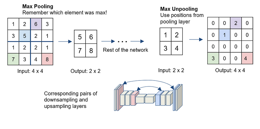
Max-Unpooling Upsampling
In summary, we need upsampling in CNNs to recover lost spatial information, generate high-resolution outputs, and improve the performance of the network. Upsampling can be performed using various techniques, and the choice of method depends on the specific task and the architecture of the network.
6) What does a 1×1 convolutional layer do?
- Dimensionality Reduction: One common use of a 1×1 convolutional layer is to reduce the number of channels in the input feature maps. By applying a set of 1×1 filters, the layer performs a linear combination of the input channels, resulting in a reduced number of output channels. This reduction in dimensionality helps reduce computational complexity and model size while still preserving important features.
- Non-linearity Introduction: While individual 1×1 convolutions are linear operations, when combined with an activation function (e.g., ReLU), they introduce non-linearity into the network. This non-linearity enables the network to learn complex and nonlinear relationships between channels.
- Feature Combination and Interaction: The 1×1 convolutional layer can also be used to combine and interact features from different channels. By applying a set of filters to the input channels, the layer computes weighted sums of the input features, allowing for feature fusion and capturing cross-channel interactions.
- Network Capacity Control: The number of 1×1 filters in the layer can be adjusted to control the network’s capacity and complexity. Increasing the number of filters increases the expressive power of the layer, allowing for more complex feature combinations and transformations.
- Adaptation and Transformation: A 1×1 convolutional layer can adaptively transform feature maps by learning a set of weights for each output channel. This allows the network to adaptively adjust the importance of different input channels for a particular task.
To recap, 1X1 Convolution is effectively used for
1. Dimensionality Reduction/Augmentation
2. Reduce the computational load by reducing parameter map
3. Add additional non-linearity to the network
4. Create a deeper network through the “Bottle-Neck” layer
5. Create a smaller CNN network that retains higher degree of accuracy
7) Purpose of pooling in CNNs? What happens when you use max-pooling instead of average pooling? When should we use one instead of the other? What happens when pooling is removed completely? What happens if we replace a 2 x 2 max pool layer with a conv layer of stride 2?
The purpose of pooling in Convolutional Neural Networks (CNNs) is to reduce the spatial dimensions of the input feature maps while retaining the most important information. Pooling is a down-sampling operation that helps in achieving translation invariance, reduces the computational complexity, and controls overfitting. The most common types of pooling are max pooling and average pooling.
Here are the key purposes and benefits of pooling in CNNs:
- Translation Invariance: Pooling helps in creating translation invariance, which means the network becomes less sensitive to the exact position of features in the input. It allows the network to detect the presence of important features regardless of their precise location within the feature maps. This property helps the model to generalize better to slightly shifted or translated versions of the input data.
- Spatial Dimension Reduction: Pooling reduces the spatial dimensions of the feature maps, which is crucial for processing high-resolution images and large input sizes. By subsampling the feature maps, the computational cost of subsequent layers is reduced, making the network more efficient and faster to train.
- Feature Selection: During pooling, only the most relevant and significant features are retained while discarding less important information. Max pooling, for example, keeps the maximum value within each pooling window, which effectively selects the most salient features. This feature selection aids in reducing the risk of overfitting by preventing the model from memorizing noise in the data.
- Information Compression: Pooling compresses the information in the feature maps, reducing the number of parameters in the network. This property helps control model complexity and prevents excessive memory usage during training and inference.
- Hierarchical Representation: Multiple pooling layers in a CNN create a hierarchical representation of the input data. The early layers capture low-level features like edges and textures, while deeper layers capture more complex and abstract features. This hierarchical representation facilitates learning hierarchical patterns and improves the network’s ability to extract meaningful features.
- Robustness to Variations: Pooling makes the model more robust to variations in the input, such as changes in object size, orientation, or position. By subsampling and retaining important features, the network can focus on capturing higher-level patterns and structures rather than being sensitive to minor input changes.
In summary, pooling in CNNs serves as a crucial operation for dimensionality reduction, feature selection, translation invariance, and creating hierarchical representations. It helps the network efficiently process large input data, improves generalization, and enhances the model’s ability to recognize patterns in real-world data.
Max Pooling
Pooling with the maximum, as the name suggests, retains the most prominent features of the feature map.
Average Pooling
Pooling with the average values. As the name suggests, it retains the average values of features of the feature map.
When using max-pooling, the maximum value within each pooling window is selected and passed on to the next layer. In contrast, average pooling takes the average value of the pooling window.
Max-pooling is typically used in convolutional neural networks to capture the most important and salient features in the input image while discarding less relevant information. By selecting only the maximum value in each pooling window, max-pooling creates a more robust representation of the image’s features, making it more resilient to variations in the input.
However, max-pooling can also lead to loss of information, as it discards all values except for the maximum, which can result in a loss of spatial resolution. On the other hand, average pooling preserves more spatial information, but it may not capture the most important features of the image as effectively as max-pooling. The choice of pooling method depends on the specific task and the nature of the input data.
Max-pooling is typically used to extract the most salient features from the input image and preserve the strongest activations while reducing the spatial dimensions of the feature map. It is useful when the goal is to detect the presence or absence of certain features in the image. For example, in object detection tasks, max-pooling can be used to detect the presence of objects of interest in the image.
On the other hand, average pooling is useful when the goal is to obtain a rough estimate of the activations across the feature map. It is particularly useful in tasks such as semantic segmentation, where the goal is to classify every pixel in the image into different classes. Average pooling can be used to aggregate the features of neighboring pixels and create a smoother output.
In summary, max-pooling is useful when the focus is on detecting the presence of specific features, while average pooling is useful when the goal is to obtain a rough estimate of the activations across the feature map. However, both techniques can be used interchangeably depending on the requirements of the task at hand.
Max Pooling – The feature with the most activated presence shall shine through.
Average Pooling – The Average presence of features is reflected.
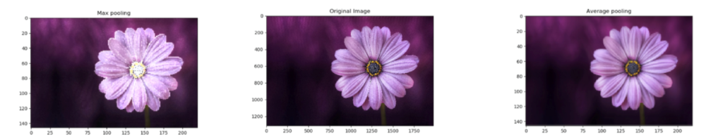
As you may observe above, the max pooling layer gives a more sharp image, focused on the maximum values, which for understanding purposes may be the intensity of light here whereas average pooling gives a more smooth image retaining the essence of the features in the image.
=========================
- Max-pooling is generally preferred when the goal is to detect the presence of a feature in an image or classify an object. This is because max-pooling preserves the most salient features by selecting the highest activation values from each pooling region.
- Average pooling is often used for tasks that require an understanding of the overall image content, such as image captioning or sentiment analysis. Average pooling gives equal importance to all regions of the image and can help to reduce the effect of noise.
- Another factor to consider is the size of the pooling window. Larger pooling windows tend to be more effective with max-pooling because they help to preserve the overall structure of the image. In contrast, smaller pooling windows are often used with average pooling to capture more fine-grained details in the image.
- It’s worth noting that recent research has explored alternative pooling techniques, such as global average pooling and fractional pooling, which can offer improved performance in certain contexts. Therefore, it’s important to experiment with different pooling methods and window sizes to determine the most effective approach for a given task.
When pooling is removed completely, the output of the convolutional layer is passed directly to the next layer without any reduction in spatial dimensions. This means that the number of feature maps in each layer remains the same as the input layer. The lack of pooling can result in a larger number of parameters and a more computationally expensive model. However, the absence of pooling can also result in a more detailed representation of the input data, which may be beneficial for certain tasks, such as object detection, where fine-grained spatial information is important.
Removing pooling entirely is sometimes done in fully convolutional neural networks (FCNs), where the objective is to generate a dense output that is spatially consistent with the input. For example, in image segmentation tasks, FCNs take an input image and generate an output mask with the same spatial resolution as the input image, where each pixel in the output mask corresponds to a label in the input image. In these cases, the lack of pooling helps to preserve the spatial information necessary for accurate segmentation.
In essence, max-pooling (or any kind of pooling) is a fixed operation, and replacing it with a strided convolution can also be seen as learning the pooling operation, which increases the model’s expressiveness ability. The down side is that it also increases the number of trainable parameters, but this is not a real problem in our days.
There is a very good article by JT Springenberg, where they replace all the max-pooling operations in a network with strided-convolutions. The paper demonstrates how doing so, improves the overall accuracy of a model with the same depth and width: “when pooling is replaced by an additional convolution layer with stride r = 2 performance stabilizes and even improves on the base model”
https://stats.stackexchange.com/questions/387482/pooling-vs-stride-for-downsampling
8) When we replace a normal convolutional layer with a depthwise separable convolutional layer, the number of parameters can go down. How does this happen? Give an example to illustrate this.
Depthwise separable convolutional layer is a type of convolutional layer in a neural network architecture that is designed to reduce the computational complexity of standard convolutional layers while maintaining similar levels of accuracy.
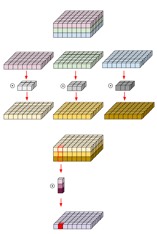
In a depthwise separable convolutional layer, the convolution operation is decomposed into two separate operations: depthwise convolution and pointwise convolution.
- Depthwise convolution applies a single filter to each input channel separately. This means that for input with C channels and a filter size of KxK, the depthwise convolution will apply C filters, each with a size of KxK, resulting in C output channels.
- Pointwise convolution, on the other hand, applies a 1×1 convolution (also known as a pointwise convolution) to the output of the depthwise convolution, allowing linear combinations of the output channels to be computed. This operation is similar to a fully connected layer, but is applied after the depthwise convolution to reduce the number of channels.
By using depthwise separable convolutional layers, the number of parameters and computations required to train a neural network can be significantly reduced, resulting in a faster and more efficient model without sacrificing accuracy.
A depthwise separable convolutional layer is a type of convolutional layer that reduces the number of parameters required to train a convolutional neural network (CNN). It is composed of two distinct layers: a depthwise convolution and a pointwise convolution.
In a depthwise convolution, the input channels are convolved separately with their corresponding kernel channel, creating a feature map for each input channel. This step is followed by a pointwise convolution, where the feature maps are combined using a 1×1 convolution to generate the final output. The depthwise convolution essentially reduces the number of input channels, while the pointwise convolution increases the number of output channels.
By using depthwise separable convolutions, the number of parameters required to train the model is reduced significantly, making the model more efficient and faster to train. This is particularly useful for mobile and embedded devices, where computational resources and memory are limited. Additionally, depthwise separable convolutions have been shown to improve the accuracy of CNNs on certain tasks, such as image classification and object detection.
In a depthwise separable convolutional layer, the convolution is separated into two stages: a depthwise convolution followed by a pointwise convolution. The depthwise convolution applies a separate filter to each input channel, while the pointwise convolution applies a 1×1 filter to combine the outputs of the depthwise convolution. This results in fewer parameters because the depthwise convolution uses fewer filters (equal to the number of input channels), and the pointwise convolution uses fewer output channels.
Goal:
Conventional Conv: Depthwise Conv + Pointwise Conv
https://towardsdatascience.com/a-basic-introduction-to-separable-convolutions-b99ec3102728
9) Can you use a base model trained on ImageNet (image size 256 x 256) for an object classification task on images of size 320 x 360? How?
Yes, you can use a base model trained on image size 256 x 256 for an object classification task on images of size 320 x 360. However, you need to make some adjustments to ensure that the model can handle the larger image size.
One approach is to use image resizing or scaling. You can resize the images/Crop to the same size as the input size of the base model, which is 256 x 256. This can be done using various image processing libraries like OpenCV or PIL in Python. However, this approach may result in a loss of some details and resolution in the larger images, which may affect the performance of the model.
Another approach is to fine-tune the base model on the new image size of 320 x 360. This involves retraining the last few layers of the base model on the new image size to adapt it to the new data. Fine-tuning can be done using transfer learning techniques in deep learning frameworks like TensorFlow or PyTorch. Fine-tuning the model on the new image size may result in better performance since the model is now trained specifically on the new image size.
In summary, you can use a base model trained on image size 256 x 256 for an object classification task on images of size 320 x 360 by either resizing the images or fine-tuning the model on the new image size. The choice of approach depends on the specific requirements and constraints of the task at hand.
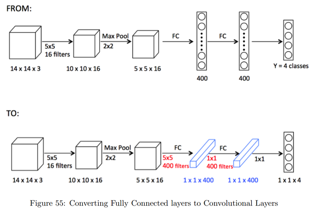
11) How can a fully-connected layer be converted to a convolutional layer?
A fully-connected layer can be replaced by a convolutional layer with the same number of trainable parameters by using a 1×1 convolutional layer. This technique is known as a “network in network” approach.
The idea behind this is that a 1×1 convolutional layer acts as a fully-connected layer when applied to the output of a previous convolutional layer. Specifically, a 1×1 convolutional layer with a depth equal to the number of neurons in the fully-connected layer can be used to replace the fully-connected layer.
For example, if we have a fully-connected layer with 512 neurons, we can replace it with a 1×1 convolutional layer with a depth of 512. The input to the convolutional layer would be the output of the previous layer, which is typically a 3D tensor with dimensions (height, width, depth). The convolutional layer would apply a set of 1×1 filters to this tensor, producing a new 3D tensor with dimensions (height, width, 512).
The resulting output tensor can then be passed on to the next convolutional layer in the network. The advantage of using a 1×1 convolutional layer over a fully-connected layer is that it preserves the spatial structure of the input, which can be important for image-related tasks. Additionally, using 1×1 convolutions can reduce the number of parameters in the model, which can help with overfitting and improve training speed.
12) Pros and cons of FFT-based convolution and Winograd-based convolution.
FFT-based convolution and Winograd-based convolution are two approaches for accelerating the computation of convolutional neural networks.
FFT-based convolution involves computing the convolution in the frequency domain using the Fast Fourier Transform (FFT). This approach can be faster than traditional convolution for large filter sizes, as it reduces the number of computations required to perform the convolution. The downside of this approach is that it requires transforming the input data into the frequency domain, which can be computationally expensive.
Winograd-based convolution involves approximating the convolution operation with a smaller set of matrix multiplications and additions. This approach can be faster than traditional convolution for small filter sizes, as it reduces the number of computations required to perform the convolution. The downside of this approach is that it requires additional precomputation to generate the matrix transformation, which can be expensive.
Both FFT-based convolution and Winograd-based convolution are methods for speeding up the computation of convolutional neural networks. The choice of which method to use depends on the specific network architecture and hardware being used.
FFT-based convolution and Winograd-based convolution are two alternative methods for performing convolution in deep learning models. Here are some pros and cons of each method:
FFT-based convolution:
Pros:
- It is faster than traditional convolution for large kernel sizes.
- It is more computationally efficient when applied to large input sizes.
- It can be used in a parallelized fashion to further improve performance.
Cons:
- It is less memory-efficient than traditional convolution.
- It is less efficient for small kernel sizes.
- It can introduce numerical instability due to the need for truncation of the Fourier transform.
Winograd-based convolution:
Pros:
- It is faster than traditional convolution for small kernel sizes.
- It is more memory-efficient than traditional convolution.
- It can reduce the number of arithmetic operations needed for convolution.
Cons:
- It requires additional preprocessing steps for the input and output.
- It can introduce numerical instability due to the need for matrix inversion.
- It is less efficient for larger kernel sizes.
In general, the choice between FFT-based and Winograd-based convolution depends on the specific application and the hardware available. FFT-based convolution is often faster for larger kernel sizes, while Winograd-based convolution is often faster for smaller kernel sizes. Additionally, FFT-based convolution is more widely used due to its relative simplicity and wider hardware support.